Computer Vision

ViT

Funnel ViT

paper

Object Detection

slides

Single Object

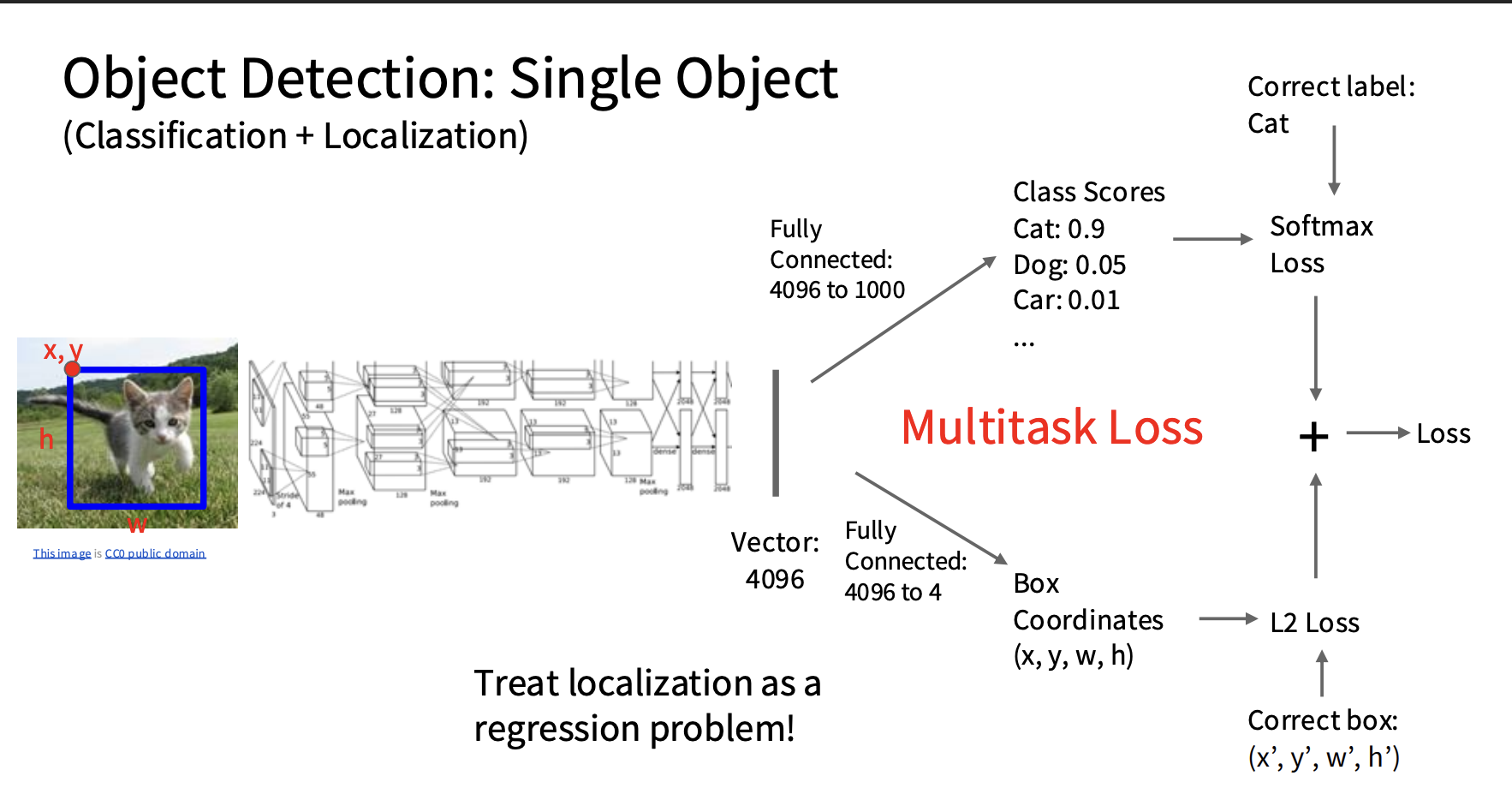
• label是：Cat + (x’, y’, w’, h')
• x, y = box 左上角的位置，w = box 宽度，h = box 高度，这些是人工标注的
• CNN把图片变成4096维向量
  • classification head：Fully connected，4096 -> 1000，输出1000个类别的分数, 做softmax
  • localization head：Fully connected: 4096 -> 4，输出predicted box = (x, y, w, h)，这些是连续值，用L2 loss
  • Total Loss = Softmax Loss + L2 Loss

R-CNN

R-CNN uses Selective Search to generate around 2000 region proposals, warps each proposal to a fixed 224×224 image, then runs a CNN on each region to classify it and later refine the box.

• Selective Search: 传统CV
• RoI: 候选的感兴趣区域

1. 生成很多 RoI
2. 图中每个 RoI 都被 crop 出来，然后 resize 成224 x 224，再分别送进 ConvNet，得到很多个feature vector
3. 每个feature vector
   • SVMs：判断这个 RoI 是什么类别(每个类别输出一个logit)
   • bbox reg：修正这个 RoI 的框, 预测(dx, dy, dw, dh)，即对之前那个框的修正

Fast R-CNN

1. 先对整张图片做 CNN backbone，得到一张 spatial feature map。

   • feature map 仍然保留大致位置信息，不是一个 single vector。

2. 用 external proposal method 得到 RoIs。

   • 在原始 Fast R-CNN 里，RoI 通常来自 Selective Search。
   • 注意：RPN 是 Faster R-CNN 的改进，不属于原始 Fast R-CNN。

3. 把每个 RoI 映射到 feature map 上，然后用 RoI Pooling 做 crop + resize。

   • 不同 RoI 在 feature map 上大小不同。
   • RoI Pooling 把每个 variable-size RoI feature 变成固定大小，比如 7×7。
   • 这样后面的 per-region head 可以处理所有 RoI。

4. 对每个 RoI feature 做两个预测：

   • classification: softmax 分类，判断 object category / background
   • bbox regression: 预测 box offsets，修正 proposal box

5. Fast R-CNN 的核心加速：

   • R-CNN 是每个 RoI 单独跑 CNN。
   • Fast R-CNN 是整张图只跑一次 CNN，然后所有 RoI 共享同一张 feature map。

Faster R-CNN

• Faster R-CNN = Fast R-CNN + RPN
• 它用 RPN 替代 Selective Search，让 proposal generation 也变成 learnable。

Region Proposal Network

• RPN 在 backbone feature map 上滑动。

• 在每个 feature map location 放多个 anchor boxes。

  • anchor box = 提前定义好的默认框
  • 每个位置可以有多个尺度 / 长宽比的 anchors

• 对每个 anchor，RPN 预测：

  • objectness: has object / no object
  • box offset: anchor 应该怎么移动和缩放，才能更接近 GT box

• RPN 只生成 proposals，不负责最终类别分类。

  • 它只判断 object vs background。
  • 真正的 category classification 由后面的 Fast R-CNN head 完成。

mask R-CNN

Mask R-CNN 在 Faster R-CNN 基础上，加了一个 mask head，负责输出这个 RoI 内部，哪些像素属于 object，哪些像素是背景

1. CNN 提取整张图的 feature map,
2. RPN 在 feature map 上生成 candidate boxes / RoIs
3. RoIAlign:把每个 RoI 从 feature map 上裁出来，并变成固定大小 [14,14], 这是该RoI的spatial feature map
4. 对每个 RoI，

   • 模型预测：

     • C 个 class scores
     • 4 * C 组box refinement。C个class, 每个class预测(dx, dy, dw, dh)

   • RoIAlign outputs a fixed-size RoI feature, e.g. 256 × 14 × 14.

   • The mask head first uses several conv layers to process this RoI feature while keeping the spatial size 14×14.

   • Then a transposed convolution / learnable upsampling layer with stride 2 doubles the spatial resolution:

     • 256 × 14 × 14 -> 256 × 28 × 28

   • Finally, a 1×1 conv maps channels from 256 to C:

     • 256 × 28 × 28 -> C × 28 × 28

   • The output is one 28×28 binary mask per class.

single-stage detector

1. 图片分成S × S个grid
2. 每个grid有三个base boxes， B=3，分别是长宽大小不同的anchor box
3. Within each grid cell: Regress from each of the B base boxes to a final box with 5 numbers: (dx, dy, dh, dw, confidence). Predict scores for each of C classes

YOLO

For each box output:

• P(object): probability that the box contains an object
• B bounding boxes (x, y, h, w)
• P(class): probability of belonging to a class

NMS: Non-Maximum Suppression

对于一个object，可能有很多的框都在predict这个object. 需要删除掉重复的框

1. 对所有 predicted boxes 按 confidence / class score 从高到低排序。
2. 先保留分数最高的 box。计算它和其他 boxes 的 IoU。
3. 如果其他 box 和它的 IoU 太高，比如 IoU > 0.5，说明它们大概率在检测同一个 object，就删除低分的 box。
4. 重复这个过程，直到处理完所有 boxes。

Object Detection with Transformers: DETR

• DETR = Detection Transformer，把 object detection 建模成 set prediction。

• Pipeline:

  • image -> CNN backbone -> feature map
  • flatten feature map into image tokens
  • add positional encoding
  • Transformer encoder 处理 image tokens，让每个位置看到全局上下文
  • Transformer decoder 接收一组 learned object queries
  • 每个 object query 在 Transformer decoder 里 cross-attends to encoder output image features，最后 decoder 输出一个 query representation。这个 representation 再接 class head 和 box head，输出一个 object prediction。

• Object queries:

  • 可以理解成固定数量的 object slots，比如 100 个 slots
  • 每个 query 最后输出：
    • class logits: bird / dog / car / … / no-object
    • box coordinates: (cx, cy, w, h)
  • 如果图里只有 2 个 objects，那么只有 2 个 queries 应该预测真实物体，其他 queries 应该预测 no-object

• Bipartite matching loss:

  • DETR 输出很多个预测框，但 GT boxes 没有顺序，所以需要对 predictions 和 GT 一一配对。
  • 每个 predicted box 和每个 GT box 算 matching cost。
  • matching cost = classification cost + box L1 cost + GIoU cost
    • IoU measures overlap between predicted and ground-truth boxes.
    • GIoU 不只看 overlap，还看两个框离得远不远。
  • Hungarian algorithm:
    • 不是贪心地每个 GT 找最近的 prediction
    • 而是找一个全局最小 cost 的 one-to-one assignment

• 配对后训练:

  • matched predictions:
    • class loss
    • box L1 loss
    • GIoU loss
  • unmatched predictions:
    • no-object classification loss
    • 不算 box loss，因为它们没有对应的 GT box

Self-supervised learning

231n lecture 12

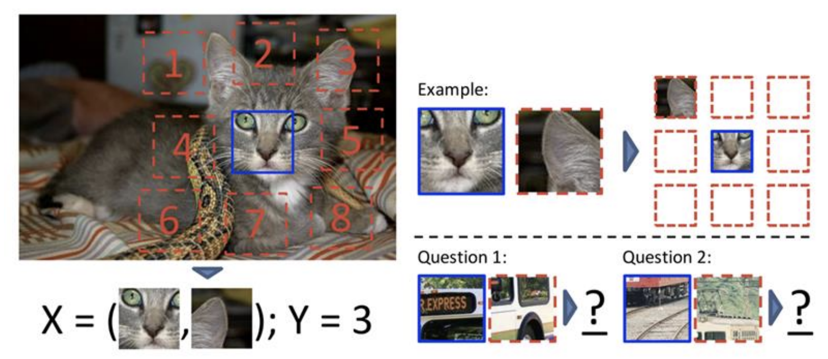
Pretext tasks from image transformations

Pretext task：不是最终任务，而是为了训练 encoder 设计的代理任务

• rotation：让模型去学判断这个图片被旋转了多少度。4-way classification
• predict relative patch locations：8-class classification task
• Inpainting:

  • 拿一张完整图片 x，人为遮住一块，得到 corrupted image。

  • 输入 corrupted image，让模型预测被遮住区域的 pixels。

  • 原图中被遮住的那一块就是 target，所以不需要人工 label。

  • 有两个 model:

    • F: inpainting model / generator，用来补全缺失区域。
    • D: discriminator，输出“这张图是真图”的概率。

  • 训练方式是交替训练：

    1. 先用 F 生成补全后的 fake image。
    2. 训练 D： 用 BCE loss 分辨 real image 和 fake image。 real image label = 1 fake image label = 0
    3. 再训练 F： loss = reconstruction loss + adversarial loss。 reconstruction loss 让补出来的 pixels 接近真实 pixels。 adversarial loss 让补出来的图骗过 D，让 D(fake) 接近 1。

  • Reconstruction loss: 只在 masked region 上算预测 pixels 和真实 pixels 的差距。 目标是内容要对。

  • Adversarial loss: 本质是 BCE / GAN loss。 对 D 来说：学会分辨 real/fake。 对 F 来说：学会生成让 D 以为是真的 fake image。 目标是视觉上更真实、更不模糊。

Contrastive representation learning

loss: infoNCE

SimCLR

1. 对同一张image,randomly做两种不同的augmentation，得到x̃_i 和 x̃_j. 训练时让他们的embedding靠近
2. 用同一个 encoder f 提取feature, 得到 h_i 和 h_j
3. 用 projection head g 得到 z_i 和 z_j
4. 对z做infoNCE loss
5. 训练完之后，用h做representation

• h中可以保留颜色、纹理细节。z中主要保留semantic信息，用来训练

1. 每一个batch有N张图片，通过augmentation得到2N张图片
2. 对每张图片，有一张positive, (2N-1)张negative
3. 算loss的时候，算两个方向L = 1/(2N) Σ_{k=1}^N [ l(2k-1, 2k) + l(2k, 2k-1) ]

Gen

Definition

Discriminative Model

给定一个输入 x，它属于哪个 label y。数学上就是学：p(y | x)。
比如给一张cat image, 输出cat/dog label
No way to handle unreasonable inputs

Generative Model

学习：这张图片本身有多像真实世界里会出现的图片？即p(x) = 这张图片的合理程度
Model can “reject” unreasonable inputs by giving them small probability mass.

Conditional Generative Model

学习p(x | y)，比如p(image | “cat”)， 即给定条件是 cat，哪些图片像猫？

Gen Models

Explicit Density

模型显式地建模 p(x)，所以可以对一个输入 x 计算它的概率/likelihood。

Autoregressive models

• 真的可以计算出prob,而不只是估计
• 把 x 拆成 sequence，然后每一步根据前面的内容预测下一个元素。因此它能用chain rule显式计算 p(x)。
• LLM是Autoregressive models
• 也可以用来生成图片。
  • pixel cnn: 给定前面的 pixels，现在这个 pixel 的值应该是多少？因为每个像素点是3 channel的0-255取值，cnn生成一个256 维 softmax，代表下一个pixel的值的概率分布
  • p(x) = p(x1) * p(x2 | x1) * p(x3 | x1, x2) * …，可以学习整张图片的概率

Approximate density

想建模 p(x)，但只能近似计算。
用一个隐藏空间 z 表示数据背后的因素，再从 z 生成 x

(Non-Variational) Autoencoders

• Autoencoder 是一个 reconstruction problem。
• 输入图片 x，经过 Encoder 得到 latent representation z，再经过 Decoder 重建出 x_hat。
• x -> Encoder -> z -> Decoder -> x_hat
• loss = ||x_hat - x||^2，也就是让重建图像尽量接近原图。
• backprop 会同时更新 Encoder 和 Decoder 的参数；可以把 Encoder 理解成模型前半部分，Decoder 理解成模型后半部分。
• 中间的 z 是 learned representation / compressed feature。
• 如果 z 有 bottleneck，例如维度较小，模型就被迫保留对重建最有用的信息，所以 z 可能学到 object identity、appearance、scene layout 等因素。

问题: 普通Autoencoder的逻辑是，如果我们可以生成一个z,然后用decoder就可以生成一个图片。但关键在于，很难学会生成一个有意义的z

VAE

Variational Autoencoders (VAE) define an intractable density that we cannot explicitly compute or optimize

But we will be able to directly optimize a lower bound on the density

• training data: x
• intuition: maximize pθ(x)，也就是在当前模型 pθ 下面，这些 training images 被生成出来的概率 / density

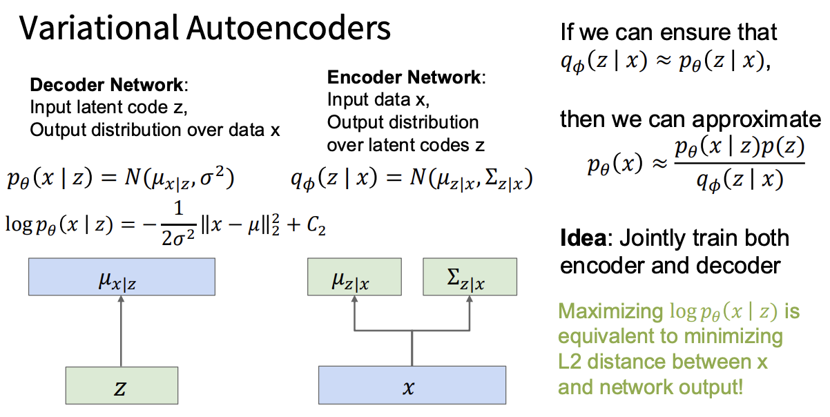
• decoder:

  • input z, output μ_{x|z}
  • learn pθ(x | z) = N(μ_{x|z}, σ²)
  • if image: 28*28 pixels, then output 784 means，生成图片的时候通常直接用means了
  • 假设所有 pixel 用同一个固定 variance σ²

• encoder:

  • learn qφ(z | x) = N(μ_{z|x}, Σ_{z|x}), which approximates p(z|x)
  • input x, output μ_{z|x}, Σ_{z|x}
  • Σ = diagonal vector, 只考虑每个pixel有自己的 variance，但不建模不同pixel之间的 correlation。

• use bayes to calculate p(x)=p(x|z)*p(z)/p(z|x)

• want to maximize p(x) <=> loss function=-log(p(x))

• training

  • 前两项叫做ELBO，第三项叫做gap. 因为KL>=0, 所以ELBO是loss的一个lower bound. 训练时，只优化前两项
  • 第一项：reconstruction term。给定一个x, 从encoder学到的分布里面sample很多z,对每个z计算log(p(x|z))，也就是把z丢给decoder, 看decoder 有多大概率重建出原来的 x,然后对这些结果取平均。这一项的目的是锻炼model的reconstruction能力，让encoder和decoder变得更好
  • 第二项：- D_KL(qφ(z|x) || p(z))。生成的时候，直接从预先规定的 z 分布，通常是 N(0, I)中，sample一些z. 这里的p(z)就是prior distribution。在训练的时候就假设p(z)服从标准高斯。这一项的目的是每个样本的 qφ(z|x) 被 regularize 到不要离 p(z) 太远.这样训练完后，我们才能直接从 p(z) sample z，再用 decoder 生成新图片。 KL代表两个distribution有多不像
  • 第三项：+ D_KL(qφ(z|x) || pθ(z|x))。注意pθ(z|x)是true posterior。代表：如果我已经看到了图片 x，那在当前decoder里，到底哪些 z 最可能生成这张 x？我们用encoder qφ(z|x)去approximate true posterior. 因为pθ(z|x) 算不出来，所以第三项算不出来

• summary： Jointly train encoder q and decoder p to maximize the variational lower bound on the data likelihood

Implicit Density

不显式计算 p(x)

Generative Adversarial Network (GAN)

slides

give up on modeling p(x), but allow us to draw samples from p(x)

1. Sample z from p(z), usually z ~ N(0, I)

2. Generate fake images: fake = G(z)

3. Sample real images x from the training dataset: x ~ p_data

4. Send both real images x and fake images G(z) to the discriminator: D(x) = probability real image is real D(G(z)) = probability fake image is real

5. Freeze Generator, update Discriminator: maximize: E_{xp_data}[log D(x)] + E_{zp(z)}[log(1 - D(G(z)))]

   In words: D should output 1 for real images, and 0 for fake images.

6. Freeze Discriminator, update Generator: sample new z ~ p(z), fake = G(z), send fake to D

   Generator wants: D(G(z)) -> 1

   In words: G wants to fool D into thinking fake images are real.

理想情况下，D(x) ≈ 0.5，代表D无法分辩Generator生成的图片是真的假的

VQGAN

VQGAN = VQ-VAE + GAN loss, 训练四个models：Encoder + Codebook + Decoder + Discriminator

• VQ: Vector Quantization, 意思是latent是离散的, 比如z=[14, 302, 81, 7, 999, …]
• codebook=[e1, e2, e3]，每个vector都是一个高维连续向量，代表一种特征. learnable parameters

1. image x 经过 encoder，得到一个 spatial latent grid z_e，比如[2,2,3],一共4个位置，每个位置是一个3-dim vector

2. 对每个3-dim vector，找 codebook 里最近的 vector，然后给这个vector起一个token id。最后这个image的feature被flatten之后变成z_tokens = [0, 1, 0, 2]

3. 查codebook, 得到 z_q（连续向量），然后喂给decoder,得到reconstructed image， x_hat

4. 让discriminator分辨real / reconstructed

为什么 VQGAN 要加 GAN loss？

如果只用 reconstruction loss，比如 L2 / MSE，重建图容易模糊，因为MSE鼓励模型输出“平均答案”。GAN loss 的作用是让重建图在视觉上像真实图片、有 sharp texture

怎么训练

A. 更新 Encoder + Codebook + Decoder
B. 更新 Discriminator

Diffusion

noise -> denoise -> denoise -> … -> image

Diffusion

cs 231n lecture 14

training

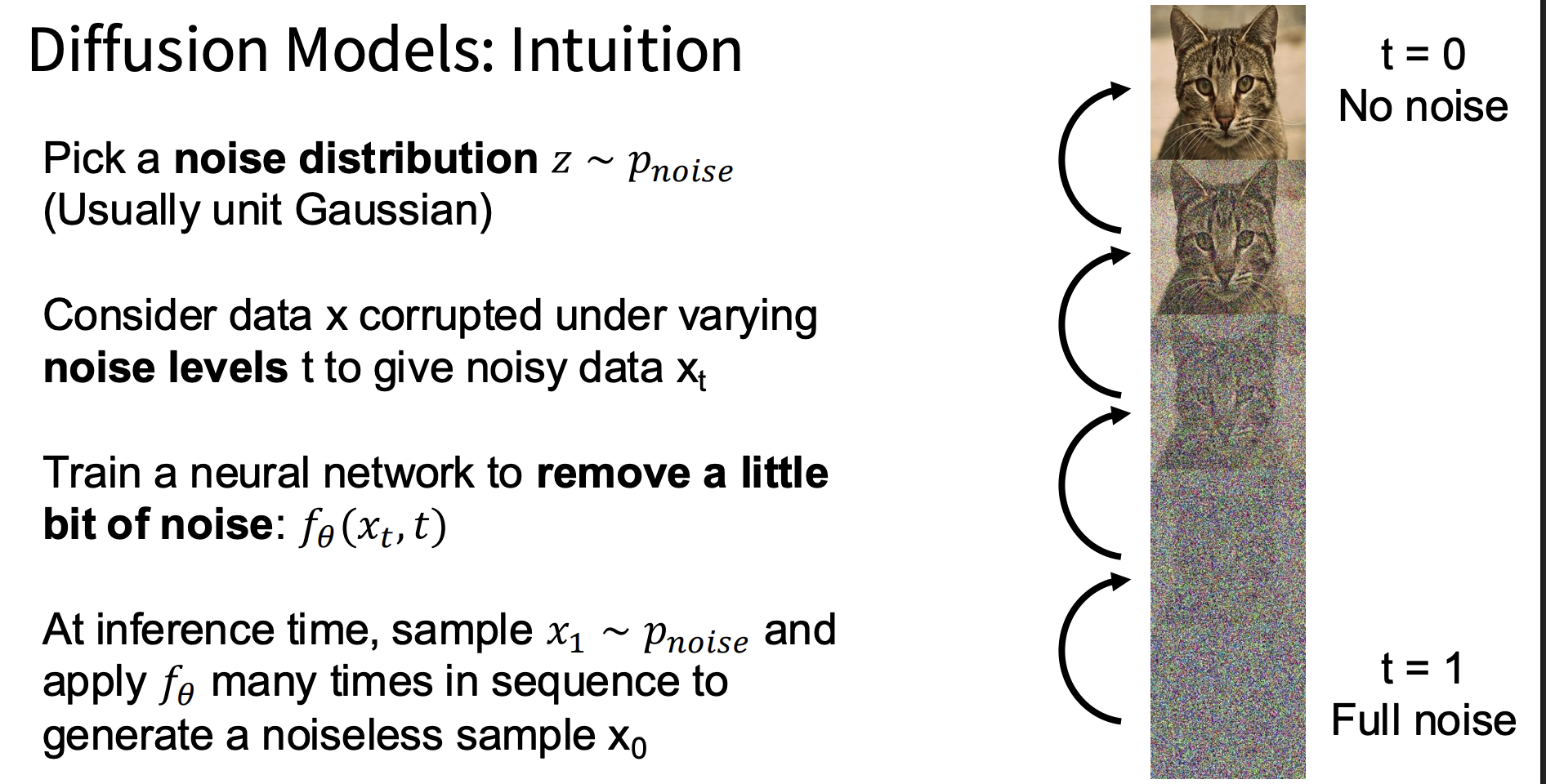
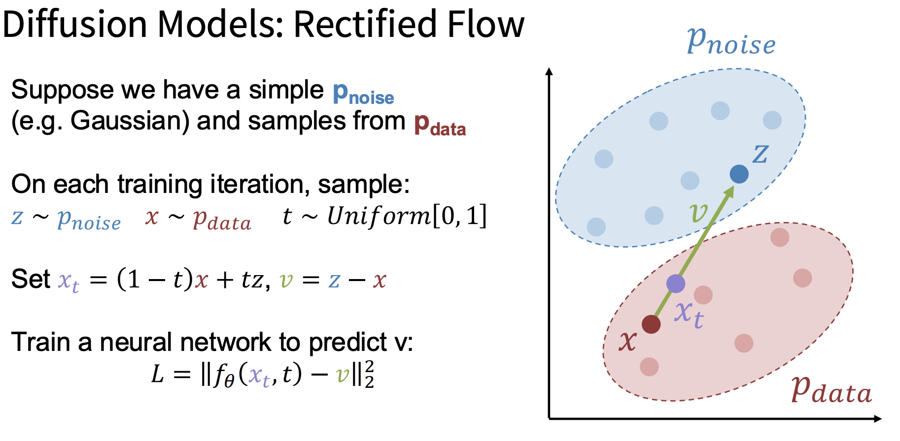
1. 从unit Gaussian里面采样一个z,代表noise
2. 采样一个真实图片x, 一个时间t, 生成从noise到真实图片，经过t时间的一张图片x_t
3. train一个NN, 让它学习预测v=z-x，也就是学从真实image到noise的方向

inference

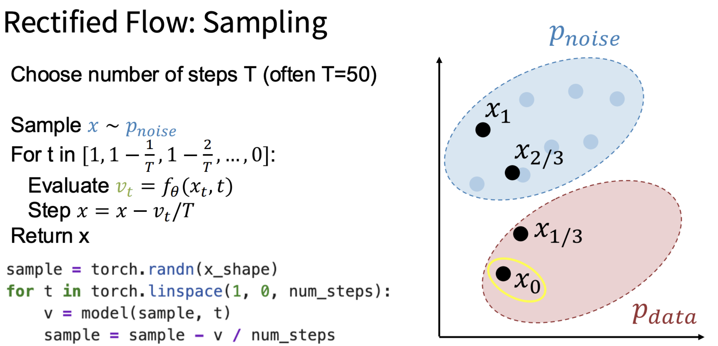
1. sample一个noise
2. 从t=1开始，用模型预测得到此时的v（输入此时的图片和t）
3. 往v的反方向走，更新图片。这就是一个去噪的过程

Conditional

从 pure noise 生成一个符合条件 y 的 data sample

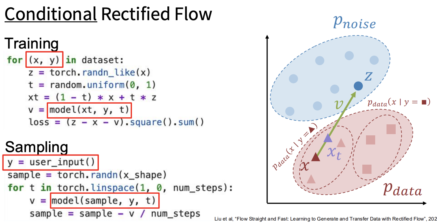
• 训练时，样本是这样的(x,y)
  • x:猫的图片
  • y:“cat”
• 大红色区域是所有真实数据：Pdata
• 但它里面可以分成很多小区域：Pdata(x∣y)
• 让模型学习，走到准确的区域去

cfg

加强prompt的约束

• 训练的时候，随机让条件y=null, 这样让model既有遵循prompt的能力，又有general生成真实图片的能力
• inference时，对某个中间图片，分别预测两个v。一个是不指定prompt的，一个是指定prompt的
• 算一下v_cfg=v_y+w*(v_y-v_null)，这个diff的意思是the direction contributed by the condition。所以这样做是为了amplify that direction to make the generation follow the prompt more strongly

Latent Diffusion Model

不要直接在原始图片 pixel 上做 diffusion，而是先把图片压缩成 latent，再在 latent 上做 diffusion，最后再 decode 回图片。

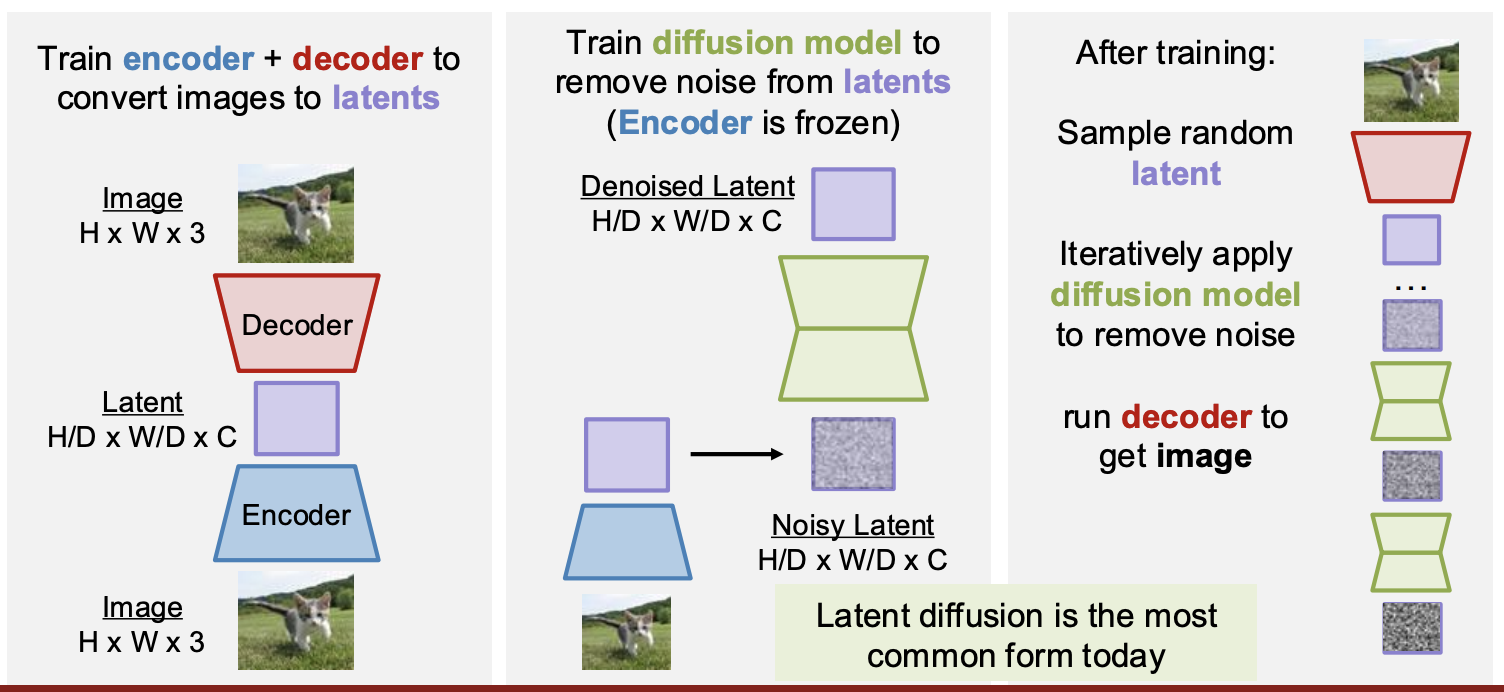
训练

• 用VAE训练一个encoder-decoder，学会latent
• 在latent上训diffusion

推理

• sample一个random latent noise
• 用diffusion给latent去除noise
• 用decoder从latent生成图片

Diffusion Transformer (DiT)

DiT 就是把 diffusion model 里面负责 denoising 的网络，从 U-Net 换成 Transformer

timestamp condition

• timestamp 进入 condition MLP，这里输出的 scale / shift，动态替代了普通 LayerNorm 里固定学习的 γ / β。
• α1, α2: 控制residual

  1 2 3

  h = AdaLN(x) attn_out = SelfAttention(h) x = x + α1 * attn_out

token condition(cross attention)

• Q: noisy image latent tokens
• K/V: text tokens

token condition(joint attention)

• 把condition token和input token拼到一起，送进Transformer

MMDiT

• image tokens 和 text tokens 各自有 modality-specific Q/K/V projection。

• image tokens -> Q_img, K_img, V_img

• text tokens -> Q_txt, K_txt, V_txt

• 然后把 Q/K/V 在 sequence dimension 上 concat： Q = [Q_img; Q_txt] K = [K_img; K_txt] V = [V_img; V_txt]

• 用 concat 后的 Q/K/V 做一次 joint attention。

• attention output 再 split 回 image stream 和 text stream。

• 最后只有 target image tokens 对应的 output 会经过 output head， 被映射成 denoising direction v。

• text tokens / reference image tokens 是 condition context， 它们参与 attention，但不会被 VAE decoder 解码成最终图片。

text-to-image

1. Text prompt 先变成 text embeddings
2. 生成一个noisy latent
3. DiT接收text embeddings和noisy latent, 输出clean latent
4. Decoder把latent还原成output image

Vision + Language

231n lecture 16