Machine Learning Basics
https://github.com/andrewekhalel/MLQuestions https://www.1point3acres.com/bbs/forum.php?mod=viewthread&tid=998257&page=1&extra= https://longxingtan.gitbook.io/mle-interview/02_ml
supervised learning
training data includes both the input features and corresponding target labels
classification
Logistic Regression
linear classification, binary classification loss function: Binary Cross-Entropy Loss


Does logistic regression have a closed-form solution?
No, there is no closed-form solution. Although the loss function is convex, taking its derivative yields a nonlinear equation containing an exponential term, so we cannot set the derivative to 0 and solve for closed-form expressions of w and b; we can only use gradient descent.
Why is it better not to use MSE as the loss?
- non-convex
- vanishing gradients
It leads to a non-convex objective and introduces an extra σ’(z) term in the gradient, which can cause vanishing gradients.
Multiclass Logistic Regression
Use softmax instead of sigmoid.

Naive Bayes
P(Y|X) = P(X|Y) * P(Y) / P(X)


Decision Tree
Supports both regression and classification.
classification
At each split, we search over all features and every possible threshold to find the split that best “cleans up” the data. Compute the Gini impurity, 1-sigma(pi^2), where pi represents the probability of each class at this split Compare this Gini impurity with the value after splitting. The larger the decrease, the more this split turns the data from “messier” into “purer”; in other words, the better the split.
For example, a node has 10 samples: 7 of class A and 3 of class B, Gini=1-(0.7²+0.3²)=0.42. If we split on “age≤30”, the left side has 6 samples, all class A, Gini=0; the right side has 4 samples, 3B1A, Gini=1-(0.75²+0.25²)=0.375, weighted Gini=(6/10)0 + (4/10)0.375=0.15, a decrease of 0.27
regression
Regression: use MSE/MAE
Parameters
- max_depth: the maximum depth of the tree, to prevent overfitting
- min_samples_split: a leaf must have at least this many samples before it can be split further
- criterion: gini / entropy / mse
Random Forest
bagging
- Bootstrap sampling with replacement: each tree uses a different training subset
- Random feature sampling: at each split, only a random subset of features is considered, reducing correlation between trees
- Individual decision trees are unpruned and grown deep; a single tree easily overfits (strong learner)
- Ensemble method: majority vote for classification tasks, averaging for regression tasks
- Overall effect: reduces model variance, mitigates overfitting; all trees are trained in parallel
boosting
- Models are trained sequentially, one after another; each subsequent tree corrects the errors of the previous tree, so it cannot be parallelized
- Core logic: continuously fit the residuals of prior models / increase the weight of misclassified samples
- Base learner: mostly uses weak learners (shallow, simple decision trees)
- Ensemble method: all models are combined with weights, rather than simple voting
- Overall effect: reduces model bias, improves overall fitting capability, more prone to overfitting
SVM
support vectors: the samples closest to the hyperplane
The goal is to find a hyperplane that maximizes the distance between the two nearest vectors from the two classes
score=w・x_i + b. Initialize w=b=0=score. Iterate over all samples (positive samples +1, negative samples -1). If we reach the first positive sample, score=0, so y_i*score=0 < 1, meaning we need to update w and b: adjust w toward the direction of the positive sample’s features and increase b, so that score gradually approaches and exceeds 1;
w = w + learning_rate*(yX - regularization_termw), b = b + learning_rate*y
For non-linearly separable data, SVM uses “soft margin” and “kernel function”.
Soft margin allows a few samples to violate the margin constraint, controlled by the C parameter; a smaller C means more tolerance.
Kernel function maps low-dimensional non-linear data to high-dimensional space, like RBF kernel, making data linearly separable in high dimension for hyperplane separation.
Hinge Loss

- Requires both correct classification and a sufficient margin
knn
- Can be used for classification, regression
- Fast training, slow prediction; suitable for small-sample scenarios
- In high-dimensional data, samples have many feature dimensions, and the distances between most samples become similar, so KNN struggles to find truly “close” neighbors. Use PCA to reduce dimensionality first.
LDA
N samples, D original features, C classes in total
- Compute the within-class scatter matrix Sw, and we want Sw to be as small as possible (samples of the same class clustered together)
- Compute the between-class scatter matrix Sb

- Perform eigenvalue decomposition on S_w^(-1)*S_b
- Sort eigenvalues from largest to smallest, and select the top k eigenvectors to form the projection matrix W(D×k)
- Multiply the original data by the projection matrix to get the reduced-dimension data (N×k)

regression
Linear Regression:
- loss=MSE
- Take partial derivatives with respect to w and b separately, and set them to 0 to get the solution
- In linear regression, if the error follows a Gaussian distribution, then minimizing MSE is equivalent to maximizing log p(y | x)

Random Forest Regression:
- Handles non-linearity, robust to outliers, no need for feature normalization
XGBoost/LightGBM (Gradient Boosting Regression):
- boosting: train a base model, then focus on the samples this model predicted incorrectly, assign these misclassified samples higher weights, and train the next model to correct the previous one’s errors; after repeating this many times, combine all the weak models together with weights
- A CART regression tree is a type of binary decision tree with only two paths: yes / no. Each leaf node outputs a continuous value. XGBoost is a strong model made up of many such trees added together sequentially.
- High performance, commonly used in industry, requires hyperparameter tuning
unsupervised learning
clustering
K-means:
- Most commonly used, simple and efficient, requires presetting the number of clusters (K), suitable for large-scale data
- Randomly select K initial cluster centers;
- Compute the distance from each sample to each center, and assign the sample to the cluster of the nearest center;
- Recompute the center of each cluster;
- Repeat steps 2 and 3 until the centers no longer change or the maximum number of iterations is reached
How to determine the value of K? Elbow Method Plot a curve with K on the x-axis and SSE (within-cluster sum of squared errors) on the y-axis; SSE keeps decreasing as K increases
Find the point where the rate of decrease suddenly slows and an “elbow” appears in the curve. The K at this elbow is a reasonably good choice
Disadvantages
- Sensitive to the initial points; different initializations give different results
- Sensitive to outliers, which can skew the mean
- Can only handle convex, spherical clusters; cannot handle irregular shapes
- Requires manually specifying K
Hierarchical Clustering:
No need to preset K; produces a tree-structured clustering result; suitable for small to medium-sized datasets
DBSCAN:
Density-based clustering, automatically identifies clusters of any shape, can detect outliers, suitable for data with uneven density
- Set ε and MinPts;
- Core point: a sample that has at least MinPts samples within its ε neighborhood;
- Density-reachable: if X is a core point and Y is within X’s ε neighborhood, then Y is directly reachable from X; if Y is within the ε neighborhood of core point Z, and Z is reachable from X, then Y is reachable from X;
- Starting from a core point, assign all density-reachable points to the same cluster;
- Points not assigned to any cluster are noise points.
GMM (Gaussian Mixture Model):
Probabilistic clustering; outputs the probability that data belongs to each cluster; suitable for soft clustering scenarios
- GMM assumes the data is generated from a mixture of K Gaussian distributions, where K must be specified in advance.
- Each Gaussian has three parameters: mean (μ), covariance matrix (Σ), weight (π) (all weights sum to 1).
- Random initialization:
- mean μ1,…,μK
- covariance matrix Σ1,…,ΣK
- weight π1,…,πK
- E
- Compute the posterior probability that each sample belongs to each Gaussian
- For each sample x, plug it directly into the Gaussian PDF to compute the density value.
- Multiply the density value by the corresponding weight to get a weighted score.
- Normalize the scores across all Gaussians to get the posterior probability that this sample belongs to the k-th Gaussian.
- M
- ① Update mean (μₖ): take the x values of all samples, multiply each by its γₖ(x) for this Gaussian, then divide by the sum of γₖ(x) over all samples.
- ② Update covariance matrix (Σₖ): also weighted by γₖ(x), compute the squared deviation of each sample x from the current μₖ, multiply by γₖ(x), then average, finally obtaining the new covariance matrix (reflecting this Gaussian’s spread and the correlation between dimensions).
- ③ Update weight (πₖ): simply take “the sum of γₖ(x) over all samples for this Gaussian” and divide by the total number of samples; this is essentially “the average weight this Gaussian holds across all samples.”
Dimensionality Reduction
PCA
Goal: find and retain the dimensions of greatest variance in the data, so that the overall variance of the data is maximized
| |
The Sigma matrix is the covariance matrix, each column of V is an eigenvector, and the Lambda matrix is a diagonal matrix whose entries are the eigenvalues, which are also the variance of each eigenvector
An unsupervised dimensionality-reduction method that uses a linear transformation to map high-dimensional data into a low-dimensional space, preserving the directions of greatest variance in the data, reducing redundancy while retaining key information.
- Standardize the data; each sample first subtracts the mean of each feature dimension. (N,D), N is the number of samples, D is the number of original features
- Compute the covariance matrix; Sigma=X_t * X, with shape (D, D),
- Perform eigenvalue decomposition on the covariance matrix to obtain the eigenvalues and eigenvectors. (D of them)
- Select the eigenvectors corresponding to the top k largest eigenvalues to form the projection matrix (D,k); K must be less than or equal to D
- Project the original data onto the k-dimensional space to obtain the reduced-dimension data. (N, K)
Why do we need to standardize the data?
If the features have different scales, features with larger variance will dominate the PCA result; after standardization, all features have consistent variance, avoiding the influence of differing scales.
How to choose the value of k?
Cumulative explained variance ratio: choose the top k eigenvalues so that the cumulative variance proportion is ≥85%-90%;
Elbow rule: plot the sorted eigenvalue curve and find the k at the “elbow” point; after the elbow, the eigenvalues decrease more slowly, meaning there is more redundant information.
Pros and cons of PCA?
Pros: good dimensionality-reduction effect, simple computation, no hyperparameters; Cons: it’s a linear transformation, so it cannot capture non-linear relationships; the reduced features have poor interpretability; and it is sensitive to outliers.
optimizer
SGD with momentum
- Helps escape local minima and saddle points
- Reduces oscillation: if the gradient in some direction is sometimes positive and sometimes negative, these gradients will partially cancel out within the momentum.
- Accelerates in the correct direction: if the gradient in some direction stays similar over many steps, these gradients keep accumulating, and the speed keeps increasing.
- Momentum accumulates historical gradients, so when the gradient direction is consistent, the accumulated momentum accelerates convergence. When there are oscillations (frequent direction changes), the opposite gradients in history will cancel out, thus reducing oscillations.
AdaGrad
- Each dimension maintains its own sum of squared gradients
- In steep dimensions, the gradient is large, so the update step size in that direction gets smaller and smaller
- Drawback: the sum of squared gradients only ever increases and never decreases, so the learning rate keeps shrinking
RMSProp
- grad_squared=decay_rate⋅grad_squared+(1−decay_rate)⋅dw∗dw
- The larger the decay_rate, the more past gradients are retained, resulting in stronger smoothing and slower change
- Solves AdaGrad’s problem of the learning rate continuously decaying to nearly 0
- RMSProp fixes AdaGrad’s shrinking learning rate by using an exponential moving average (EMA) of squared gradients instead of a cumulative sum. The decay rate (usually β2=0.9) controls how much recent gradients matter: higher β2 keeps more history, while lower β2 focuses on recent steps. This way, the denominator doesn’t keep growing indefinitely, so the learning rate remains stable over time.
Adam
- Adam = Momentum + RMSProp (Adaptive Learning Rate) + Bias Correction
- moment1 = beta1 * moment1 + (1 - beta1) * dw
- moment2 = beta2 * moment2 + (1 - beta2) * dw * dw
- moment1_unbias = moment1 / (1 - beta1 ** t)
- moment2_unbias = moment2 / (1 - beta2 ** t)
- w -= learning_rate * moment1_unbias / (moment2_unbias.sqrt() + 1e-7)
- Adam uses the first moment m_t to smooth the gradient direction, uses the second moment v_t to scale the step size for each dimension, and then uses bias correction to fix the bias introduced by initializing from 0


Neural Network
neuron
 output=sigmoid(w0x0+w1x1+w2)
This can be understood as:
output=sigmoid(w0x0+w1x1+w2)
This can be understood as:
- x0, x1 are the outputs of two neurons from the previous layer
- This represents a neuron in the output layer, e.g., a binary classification problem
Vanishing Gradients
 Gradient computation depends on: the activation function derivatives and weight matrices of later layers, as well as the output values of earlier layers
- Causes
- The activation function’s derivative is too small
- Take sigmoid as an example: its derivative has a maximum value of only 0.25, and is often much smaller than 0.25 most of the time. As a result, the earlier the layer, the closer its gradient gets to 0
- Initial weights are too small
- The activation function’s derivative is too small
- Solutions
- relu/leakyReLU: ensures the activation function’s gradient is not too small
- Batch Normalization: ensures the output values of earlier layers are not too small
- Weight initialization strategy: keeps the variance of each layer’s output consistent
- Xavier initialization: sigmoid/tanh
- He initialization: ReLU and its variants
- Xavier initialization: sigmoid/tanh
- Architectural improvements
- Residual connections
- LSTM/GRU

Exploding Gradients
- Initial weights are too large
- Gradients are too large (relu gradient=1, tanh’s gradient is close to 1 near 0)
- Solutions
- Gradient Clipping: set a threshold for the gradient, and scale it down if it exceeds the threshold
- Batch Normalization: normalizes the input of each layer so that each layer’s input has mean 0 and variance 1
- Residual Connection: ResNet’s skip connection lets the gradient take a direct shortcut, avoiding amplification from repeated multiplication
batch size vs epoch vs iteration
- epoch: one full pass through the entire training set
- batch size: the number of samples fed to the model at once in a single iteration
- iteration: one forward pass + backward pass + parameter update
Residuals
one residual block: x→Conv→ReLU→Conv→output
In ResNet, this block learns F(x)=H(x)−x, and the final output is y=F(x)+x
A skip can be added every two or three layers; for example, x->h1->h2->h3->h4 can be changed to
- h2=x+F1(x)
- h4=h2+F2(h2)

Questions
Bias-Variance Tradeoff
Error = Bias² + Variance + Irreducible Error
bagging vs boosting
- bagging: reduce variance
- boosting: reduce bias
train vs test vs val
The training set is used to train the model’s parameters, the test set is used to evaluate the final model’s generalization ability, and the validation set is used to tune hyperparameters during training
Underfitting vs Overfitting
Overfitting
- Performs well on train but poorly on test/val
- Solutions:
- Increase training data / data augmentation
- augmentation: we can rotate the image, crop parts of it, or adjust its brightness. This way, the model learns more general patterns rather than fixating on specific, unique details in the training set
- Reduce the number of layers/width of the NN
- For neural networks, we can reduce the number of layers or the number of neurons in each layer to simplify the model structure. A simpler model is less likely to memorize noise or specific details in the training data, thus reducing the risk of overfitting
- From a training perspective
- early stopping
- monitor the val loss
- weight decay: w = w * (0.999) - learning_rate * gradient
- weight decay is often implemented by multiplying the weights by a decay factor less than 1 during each parameter update, which shrinks the weights over time.
- It is one way of implementing L2, and is mathematically equivalent to it
- early stopping
- regularization
- L1: loss + λ * sum of absolute values of weights (L1 norm)
- For L1 regularization, we add a penalty term to the loss function: a regularization parameter multiplied by the sum of the absolute values of all weights
- L2: loss + λ * sum of squared weights (L2 norm). Shrinks all weights toward smaller values, but not to 0
- dropout: for example, if the dropout rate is 0.4, then only 60% of the nodes are active on each forward pass, and the forward output must be divided by 0.6. The goal is to keep the model from over-relying on certain neurons
- L1: loss + λ * sum of absolute values of weights (L1 norm)
- bagging (random forest)
- Increase training data / data augmentation
Activation Functions
Input x = [x1, x2]
Hidden layer: z1 = w1·x + b h1 = activation(z1) ← the activation function is used here
Output layer: z2 = w2·h1 + b2 y_hat = σ(z2) ← the output layer generally uses sigmoid/softmax
- sigmoid:
- Suitable for binary classification tasks and prone to vanishing gradients. Its derivative ranges from 0 to 0.25.
- σ(x)=1/(1+e^(-x))
- σ’(x)=σ(x) * (1-σ(x))
- Tanh:
- Suitable for binary classification tasks. tanh(x)=2*sigmoid(2x)-1, with values in (-1,1)
- In binary classification problems, tanh is generally used in hidden layers, while sigmoid is used in the output layer
- Relu
- relu(x)=max(0,x)
- Because its structure is simple, both forward propagation and backpropagation are much faster than sigmoid/tanh, greatly improving training speed
- Dying neurons
- leaky relu
- LeakyReLU(x)=max(αx,x)
- Gives a small slope in the negative region, so the gradient doesn’t die.
- SiLU / Swish
- SiLU(x)=x⋅sigmoid(x)
- gating: a number between 0~1. 0=off, information is not passed through; 1=fully on
- self-gating: SiLU’s gating sigmoid(x) comes from the input x itself
- smooth, does not cause dying neurons
- swiGLU
- out = (W1 x) * sigmoid(W2 x)
- One linear layer produces the features, and another linear layer produces the learnable gate
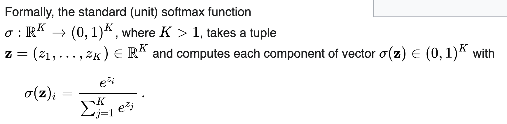
- softmax
- Multi-class classification tasks
- Converts the output into a probability distribution that sums to 1
loss function
- cross entropy
- binary
The model outputs a single logit for the positive class, then applies sigmoid to get pi. This is mathematically equivalent to outputting logits for both classes and then applying softmax
- multi class
For each sample, the model outputs a logit for each class, then applies softmax
- Why is softmax said to be a natural pairing with cross entropy?
- Because taking the partial derivative of the loss with respect to the raw output logit gives pj-yj. pj represents the predicted probability that this sample belongs to class j, and yj represents 0/1, i.e., whether the sample actually belongs to class j
- ∂L/∂z = ∂L/∂p × ∂p/∂z
- binary
- InfoNCE
- contrastive learning
- Cross entropy loss for a N-way softmax classifier
- MSE
- Regression / continuous reconstruction
- y is a continuous value, p(y|x) = Gaussian with fixed variance
- model outputs the mean
- loss = MSE
 The model outputs a single logit for the positive class, then applies sigmoid to get pi. This is mathematically equivalent to outputting logits for both classes and then applying softmax
 For each sample, the model outputs a logit for each class, then applies softmax
Class Imbalance
- data level
- Oversampling: duplicate or generate samples for the minority class, like using SMOTE to create synthetic samples.
- Undersampling: randomly remove some samples from the majority class to balance the distribution.
- loss function level
- Class Weight: We assign a higher weight to the minority class in cross-entropy loss. For example, if 990 samples are normal and 10 samples are fraud, then weight = total count / count of that class = 100; if a fraud sample is predicted as normal, the loss is 100
- Focal loss down-weights easy examples (mostly majority class) and focuses on hard ones.
The larger pt is, the more confident the model is in its prediction, and the easier this sample is
- algorithm & evaluation level
- Use models more robust to imbalance, like Random Forest, XGBoost with scale_pos_weight.
- Choose proper metrics: F1-score, AUC-ROC, AUC-PR, recall, precision instead of accuracy, since accuracy is misleading.
 The larger pt is, the more confident the model is in its prediction, and the easier this sample is
sgd
- SGD cannot be parallelized
- SGD is easier for online learning
MLE
Derive mu and sigma
normal distribution


Covariance Matrix
- A symmetric matrix whose dimension matches the data dimension; 2D data corresponds to a 2×2 matrix.
- Diagonal elements: the variance of each dimension, describing how spread out a single dimension is; the larger the value, the more spread out.
- Off-diagonal elements: the covariance between two dimensions, describing the linear correlation between dimensions.
- Meaning of positive/negative/zero covariance: positive means the two dimensions vary in the same direction; negative means they vary in opposite directions; zero means they have no linear correlation.
- Example of 2D visualization: when the covariance is 0, the contour lines of the Gaussian distribution are circular; when the covariance is positive, the contour lines form a tilted ellipse, with the distribution more concentrated in the first and third quadrants.
confusion matrix
| Predicted Positive | Predicted Negative | |
|---|---|---|
| Actual Positive | TP (True Positive) | FN (False Negative) |
| Actual Negative | FP (False Positive) | TN (True Negative) |
- Accuracy: shows how many predictions the model got right out of all the predictions. (TP+TN)/(TP+FN+FP+TN)
- Precision: the quality of the model’s positive predictions. (TP)/(TP+FP)
- Recall: measures how good the model is at predicting positives. TP/(TP+FN)
- F1-Score: combines precision and recall into a single metric to balance their trade-off. (2 * precision *recall)/(precision+recall)
Convex Function
- The function has exactly one unique global minimum overall
- No matter which point you start gradient descent from, it is guaranteed to find the global optimum, without getting stuck partway.
Data Drift
The statistical distribution of real-world data gradually changes over time/environment, becoming different from the data distribution used when training the model, causing the model to become less and less accurate the longer it is used in production
Transformer
Self-Attention
 a fluffy blue creature roamed the forest
Q
- word embedding: dim=12288. For example, creature’s embedding (E4) represents: I am creature, I am a noun, my position is xxx, and I am close to animal
- Wq: “how do I ask questions”, dim=[dim_model,dim_k]
- Q4: dim=dim_k
- Q4=E4 @ Wq
- represents the question generated by the word creature, e.g., “is there a word to describe creature”
K
- K4:
- K4 = E4 @ W_k
- I am a noun; I can be selected by a query looking for nouns
- W_K learns “how to generate the key” from each word’s embedding, so that every word’s Key vector can reflect what information it can provide
- K2: I am an adjective; I can be selected by a query looking for adjectives
- Q4 @ K2 is high (dot product, get a scalar)
- Next, every pair of words has its Q and K multiplied together, then divided by sqrt(dim_k), and softmax is applied so that each column sums to 1
V
- Vi
- Vi = Ei @ W_V
- dimension=128
- updated E4=sum(word i’s weight toward creature*Vi), dimension=128
Cross-Attention
A looks at B → two different sets of information; A goes into B to find the key content
Generally, Q is a separate query matrix, and K/V are the context matrix
Normalization
Batch Normalization
BatchNorm usually computes mean/std for each feature, along the batch dimension
Layer Normalization
LayerNorm normalizes each token’s own D features
- h_i = [h_i1, h_i2, …, h_iD], representing the i-th hidden vector output by a given layer
- μ_i = mean(h_i), σ_i = std(h_i). Then normalize: z_i = (h_i - μ_i) / σ_i, []
- Finally, apply a learnable scale and shift: y_i = γ ⊙ z_i + β. Note that both γ and β are D-dimensional; here ⊙ denotes element-wise multiplication, meaning each dimension has its own scalar and shift
Fine-Tuning
LoRA
- Generally applied to Wq and Wv
- output = Wq * x + B * A * x
- B(dim_model, rank)
- rank is small (8/16)
- The original weight matrix is frozen during training, to avoid destroying the pretrained results
SFT
- Uses manually annotated Q&A pairs for supervised training, improving answer accuracy for specific tasks
- Drawback: lacks the ability to judge “answer quality”. For example, if the labeled data contains incorrect or suboptimal answers, SFT will directly learn from them
- Tens of thousands of examples are enough, but the requirements for data quality are high
- Training data format
- Instruction: summarize the following passage
- Input: xxx
- Response: xxx
RLHF
- SFT, to obtain the model that has undergone SFT
- Train the Reward Model
- Give the SFT model the same question and have it generate several different responses
- Humans rank these responses: which is better, which is worse, which is unsafe
- Use this ranking data to train a reward model, RM
- PPO reinforcement learning
- The model generates a response
- RM scores the response
- High score → encourage the model to keep doing this
- Low score → penalize, so the model changes its behavior