Neural Network

terminology

For example, suppose there are 10,000 samples with a batch size of 100:

• epoch: all 10,000 samples go through forward + back prop once. After every epoch, the data should be shuffled to make sure each batch is made up of a different combination of samples each time.

• iteration: one iteration means 100 samples go through one forward pass (computing the loss) + backpropagation (computing the gradients), and then optimizer.step() updates the weights.

• The larger the batch size, the more accurate the gradient estimate, but the slower the convergence.

• Activation function: nonlinearity can only be introduced when an activation function is used.

• back prop umich slides

GD vs SGD

• Batch GD: the batch size is N, i.e. the full dataset. All samples are used together to do forward + backward, updating the parameters once.
• SGD(traditional): the batch size is 1; if there are 10,000 samples, the parameters are updated 10,000 times.
• mini-batch SGD: a single small batch is fast & parallelizable; the gradient estimate is noisy and the convergence trajectory jitters, but this makes it easy to escape local optima
• However, SGD does not guarantee escaping local optima

SGD’s disadvantages:

• Batch gradients can split all samples across multiple GPUs to compute simultaneously, then average the gradients. SGD’s (K+1)-th update depends on the result of the K-th update
• Once it’s already very close to the minimum, the noise makes it hard for SGD to converge more precisely, requiring a smaller learning rate or switching to full-batch gradients

optimization

The learning rate is no longer a fixed constant, but instead changes with the epoch. The decay function defines how the learning rate changes; decr represents the decay factor

first pass: SGD

• Momentum: the current update direction takes into account not only the current gradient, but also the previous update direction (weighted).
• AdaGrad: sets a separate learning rate for each parameter, adjusted as training progresses. It accumulates the sum of squared historical gradients and uses it to scale the learning rate (adaptive)
• RMSProp: an improvement over AdaGrad. It keeps the learning rate stable without decaying too quickly; converges faster
• Adam: adaptive+momentum, community fav

regularization

L1

• Drives some weights to converge to exactly 0 👉 produces a sparse model;
• Commonly used for feature selection (filtering out unimportant features);
• Not very sensitive to outliers

L2(widely used)

• Makes weights smaller, but not 0 👉 produces a dense model
• Better suited to learning complex patterns (since all features are retained)
• Downside: more sensitive to outliers (since squaring amplifies large values)

Dropout

Temporarily masks some neurons during training. In every forward pass, each neuron has a certain probability of being dropped. Doing this effectively prevents the network from over-relying on certain neurons, thereby improving the model’s generalization ability.

Usually choose either L2 or Dropout

Data Augmentation

Before the training data is fed into the model, augmentation is applied to the original images: The augmentation is redone in every epoch, generating different samples

The augmentation operations are usually applied randomly (such as random flips, random rotations)

Early Stop

When performance on the validation set stops improving, training is stopped, to prevent overfitting.

exploding/vanishing gradients

reason:

• The initial input isn’t normalized, causing the gradients computed during back prop to be too large, which then accumulates layer by layer
• Weight initialization is too large/too small remedies:
• normalize the training/testing/validation data sets
• batch normalization: for each batch, normalize each layer’s output (before ReLU)
• Weight initialization (Xavier and He), which relates the weight variance to the input/output dimensions

CNN

Term

• stride: the step size by which the convolution kernel (filter) moves across the image each time

Image Convolution

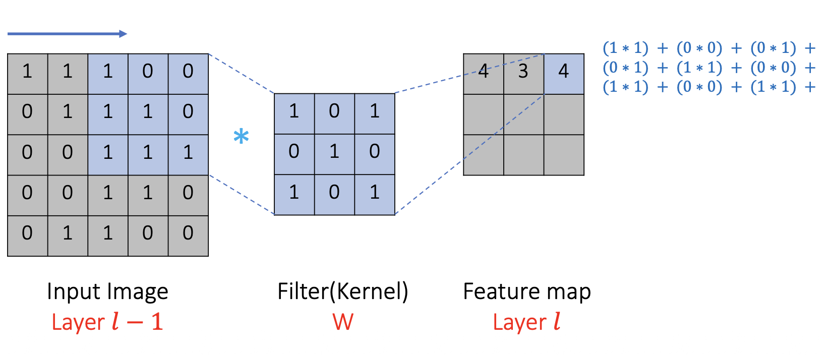Then multiply element by element

The input image passes through a filter layer to extract features; different filters serve different purposes

• identity: output image = input image
• Edge Detection: when adjacent pixels differ greatly → produces a high value (a bright edge); when adjacent pixels are similar → the result is close to 0 (a dark background); result: white lines on a black background, showing the image edges.
• Sharpen: sharpens edges

dimension

• same convolution: if you want the input and output image dimensions to stay the same, the input image must first be padded
• valid convolution: the output image dimensions become smaller

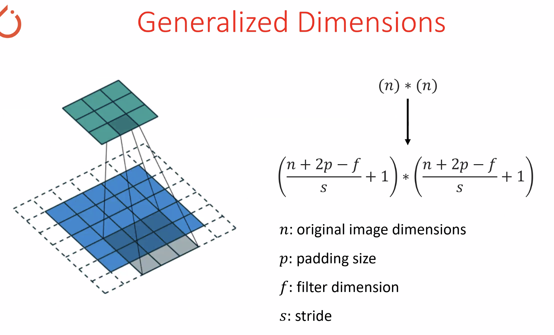
Volume Convolution

Used for processing color images; the kernel has three channels

The convolution kernel slides simultaneously across every channel of the input image. At each position, the element-wise products between the kernel and the corresponding channel are computed and then summed.

The results across the three channels (R/G/B) are then summed together (Sum).

multiple kernels? In one convolution layer, multiple different filters are used at the same time to scan the input image, in order to extract different types of features.

For example, with 5 filters, each having three channels, that’s 15 matrices in total. Each filter extracts a different image feature, and the final output is 5 feature maps

Composing CNNs

Pooling Layer

Pooling is an operation that performs downsampling on the feature map. It doesn’t introduce any new parameters; it simply takes a representative value from the input

• Improves the model’s robustness to positional changes: regardless of whether the “eye” is on the left, right, or in the middle of this small region, as long as an “eye feature” appears, the maximum value will capture it. Even if the feature shifts slightly in position, as long as it stays within this small region, the output value will be numerically similar, which makes the model insensitive to slight translations or positional changes.

CNN Advantages & Disadvantages

• translation equivariance: the same parameters can act on different positions. Whether the eye is in the top-left or bottom-right of the image, it can still be detected
• High computational cost

setting

 1
 2
 3
 4
 5
 6
 7
 8
 9
10

import torch
import torch.nn as nn

conv = nn.Conv2d(
    in_channels=3,   # Number of input channels = 3 (RGB)
    out_channels=16, # Number of output channels = 16 (i.e., 16 filters)
    kernel_size=4,   # Spatial size of each kernel = 4x4
    stride=1,        # Stride, default 1
    padding=0        # Whether to zero-pad; here we assume no padding
)

The filter size should be 1634*4, for a total of 48 filter matrices and 784 parameters Outputs 16 matrices; the result in each matrix is obtained by summing across the three RGB channels

1
2

x = torch.randn(1, 3, 28, 28) # randomly generate a 28×28 RGB image
y = conv(x) # y is the output image, with shape 1*16*25*25

When PyTorch creates a convolutional layer with nn.Conv2d(…), it automatically initializes the convolution kernel weights and bias parameters.

RNN

slides

• h_t = f(W_x x_t + W_h h_{t-1} + b): updating the hidden state requires both the old memory and the new memory
  • h_1 = f(W_x x_1 + W_h h_0 + b)
  • h_2 = f(W_x x_2 + W_h h_1 + b)
• ŷ_t = W_y h_t + b_y

Exploding Gradients

• ∂h_t / ∂h_{t-1} = f’(activate) * W_h

• ∂h_t / ∂h_{1} needs to be multiplied by W_h (t-1) times

• gradient clipping: compute the global norm over all of the model’s gradients, and if it exceeds a certain threshold, scale it down

many to many

• Every time step has an output (each h is one output y)
• The loss is the total loss, i.e. the losses from all time steps summed or averaged

sequence to sequence

• encoder: finally outputs a context vector, c=h_T, which summarizes the meaning of the entire sentence

• decoder: s_t is the current state. The current word y_t is predicted based on s_t. s_t is determined by three things:

  1. The previous output word y_{t-1}
  2. The previous decoder hidden state s_{t-1}
  3. The context vector c given by the encoder

• Problem: all the information in the input sequence must be squeezed into a single fixed-length context vector. The longer the input, the easier it is for information to get lost.

LSTM

• Uses the sigmoid and Tanh activation functions
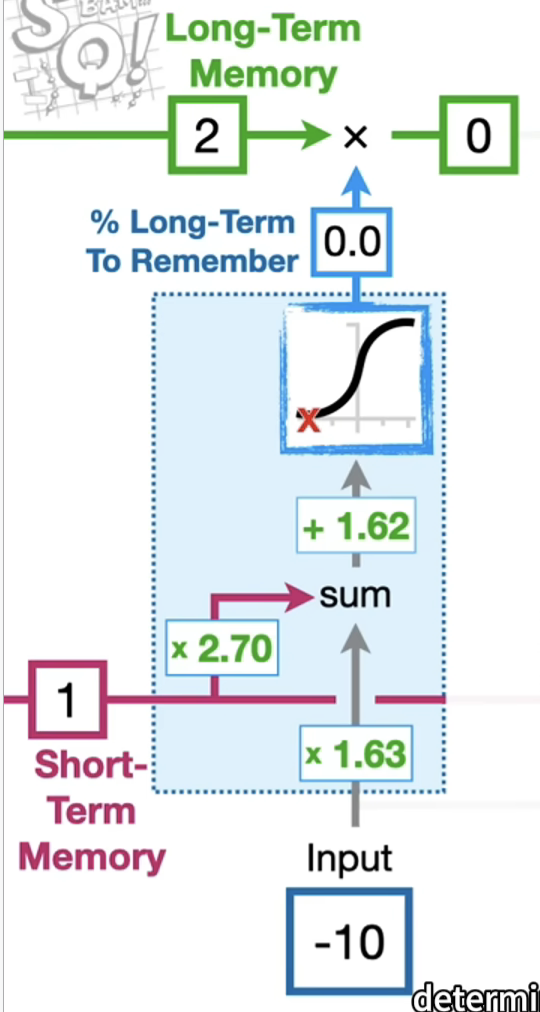
• cell state: long term memory

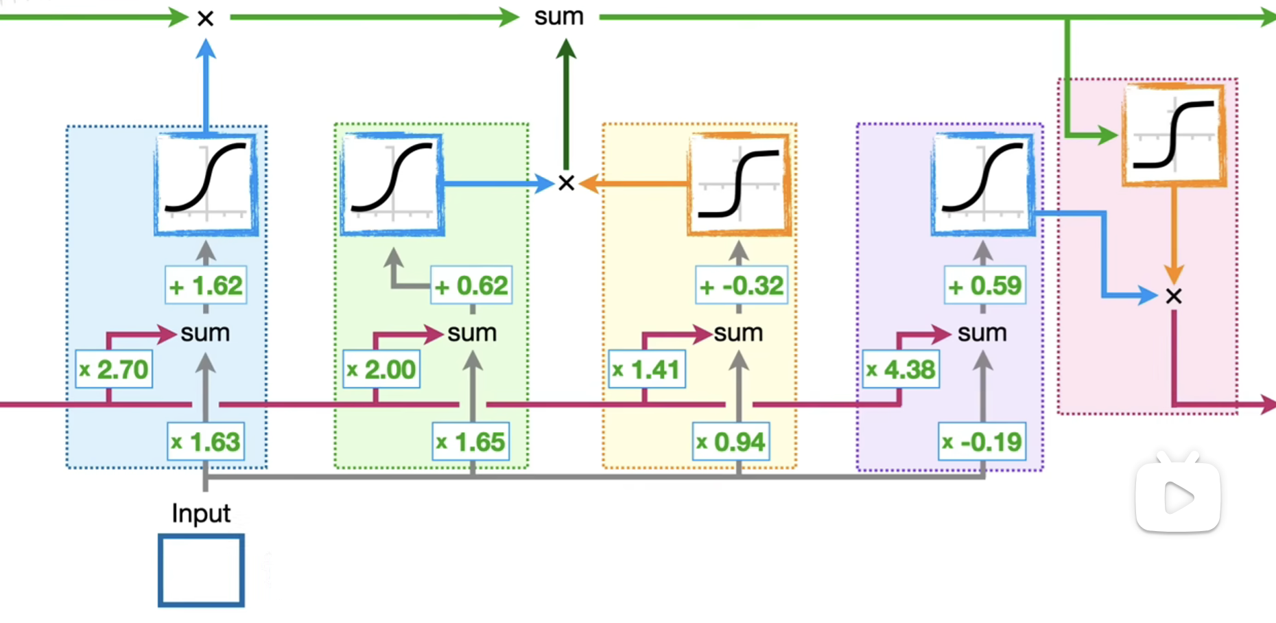
1. The short-term memory and the input are each multiplied by their weights, and the sum is taken, plus a bias value, and then sigmoid is applied. The resulting value represents the percentage of the long-term memory that is remembered; this is also called the Forget Gate
2. Step two: the block on the right here represents the potential

• The long-term memory is computed as the weighted sum of the input and the short-term memory, plus a bias, and then tanh is applied; the result is also called the candidate state.

• The result computed by the block on the left is: what percentage of the potential long-term memory is remembered. This part is called the input gate

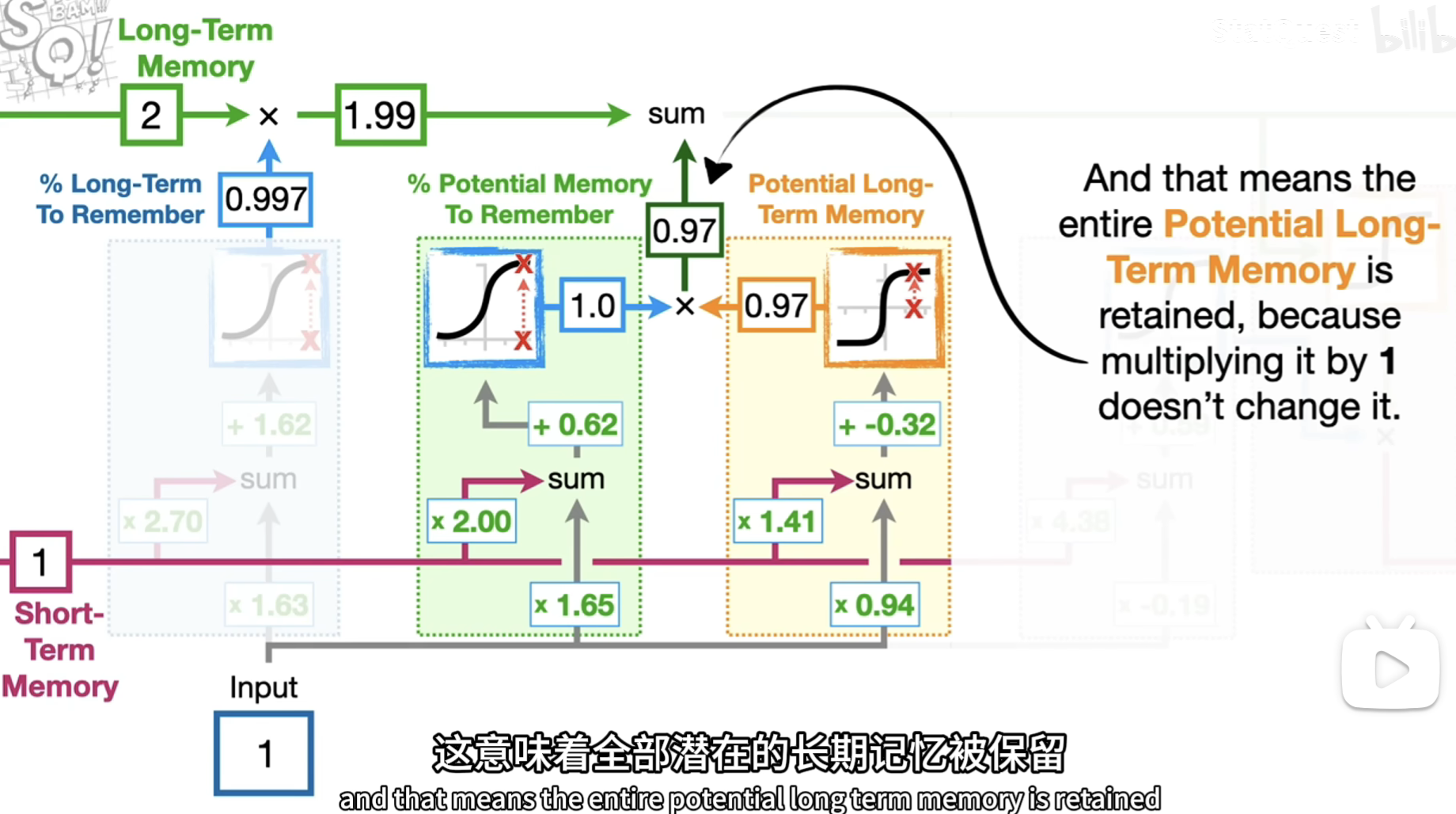
3. update short-term memory

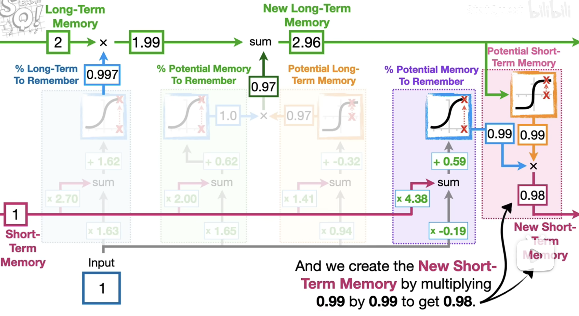
• The block on the right is the potential short-term memory. Applying tanh to the updated cell state gives this.
• The block on the left represents what percentage of the potential short-term memory we want to keep. It is likewise obtained by taking a weighted sum of the short-term memory and the input, and then applying sigmoid
• Multiplying the percentage by the potential short-term memory gives the new short-term memory, also called the output state (hidden state)

Transformer

RNN with Attention

• At every step of the decoder, a weighted context vector is computed. For every h_i, there is an attention score, e_{t,i}
• The current decoder state s_{t-1} and every encoder hidden state h_i are used to compute a matching score e_{t,i}, and then softmax is applied to obtain e_{t,i}
• Attention concept
  • Q = decoder states s_t
  • K/V = encoder states h_i
  • output = context vectors c_t

Attention

1. similarity: e[N_x]. Each q does a dot product with every piece of data, giving a similarity score; these are concatenated together to form e[N_x]
2. Scaled softmax is applied to e[N_x], giving this query’s attention weight over every piece of data
3. a[N_x] is used to take a weighted sum over the data, giving the output vector [D_x]

cross attention

1. Q:[N_q, D_q], there are multiple queries. Both K and V are learnable projections of the data X, K: [N_x, D_q], V: [N_x, D_v]. Note that V’s dimension may differ from K’s
2. Q @ K_T gives E:[N_q, N_x]; each row represents one query’s similarity to all the data, and softmax is then applied to each row, giving one query’s attention score over all the data
3. Y = A @ V, [N_q, D_v]

self attention

• masked self attention: when computing the similarity score, earlier data’s queries are not allowed to look at later v’s, i.e. the score is set to -inf

• mha: run multiple copies of the attention layer, then concatenate the results together.
• The attention layer’s input/output dimension is D; if there are H heads, then it runs the computation H times, each time with QKV dimension D_H=D/H; finally the H results are concatenated together, so the output layer’s dim is still D
• In practice, compute all H heads in parallel using batched matrix multiply operations
• When multiplying the similarity matrix by V, the time/space complexity is O(N^2). If FlashAttention is used, the space complexity is O(N)

Transformer Block

1. The first layer is a self attention layer, with matching input/output dimensions, followed by adding a ResNet connection
2. Layer Normalization, which normalizes and applies scale+shift across all dimensions of each hidden vector
3. Feed Forward: applies an MLP layer to each vector, usually two layers. MLP(x) = W2 * activation(W1 * x + b1) + b2. The dimension is expanded first, then reduced. Then a ResNet connection is added.
4. Layer Normalization

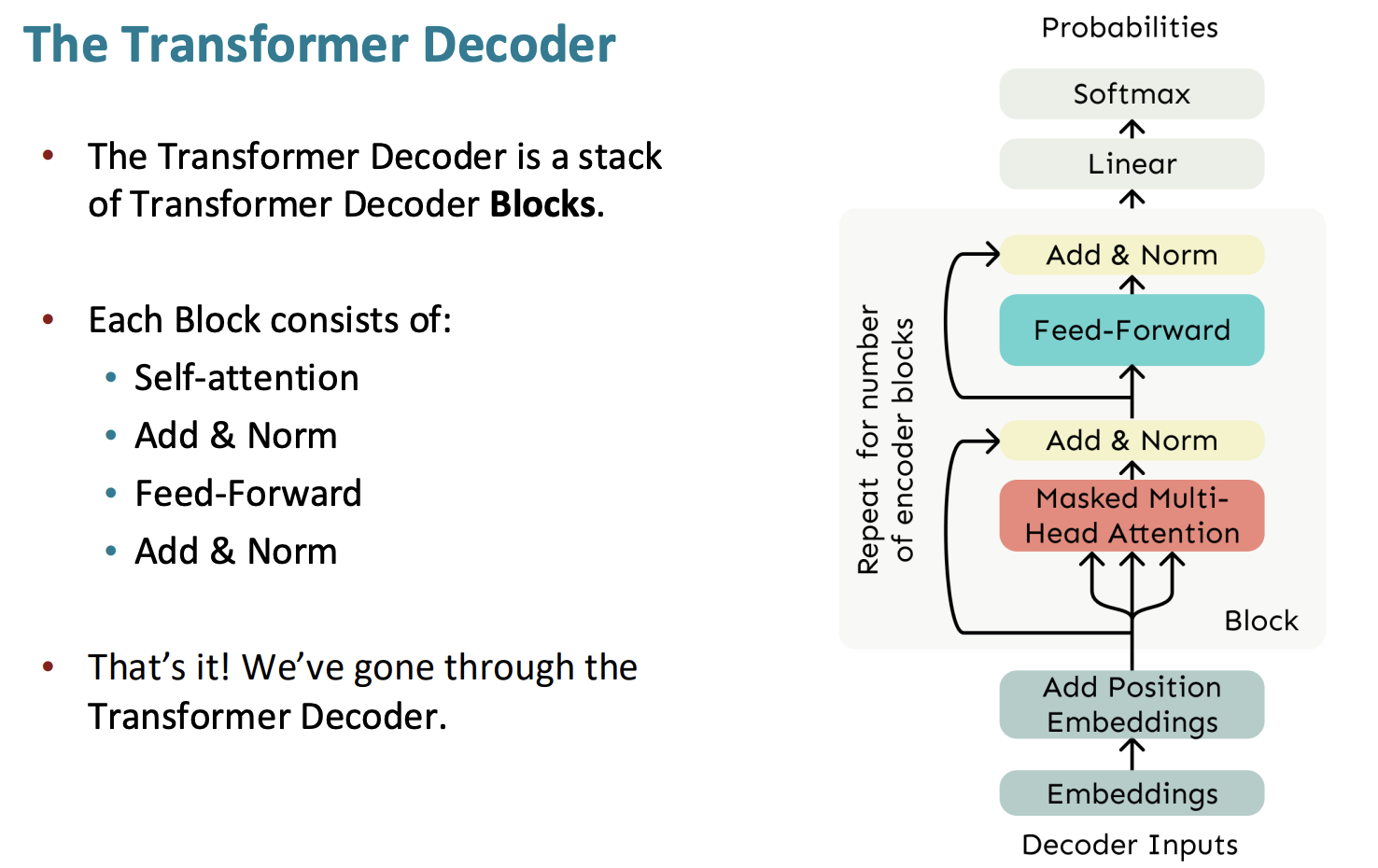
• A decoder first takes the embedding, then adds the position embedding, and then passes through multiple layers of decoder blocks
• Finally, it goes through a linear layer to obtain the probability of every possible next token

Language Model

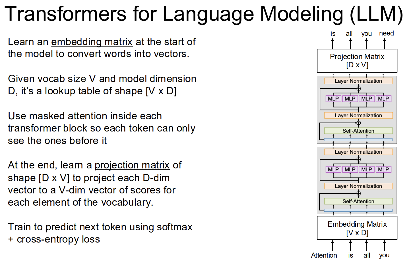This is a decoder-only Transformer, such as GPT or LLaMA

1. Learn an embedding matrix that maps tokens to vectors. If vocab size=V, dim=D, then the table is: [V, D]
2. Masked attention is used inside the transformer block
3. Learn a projection matrix.
   • The input at this step is one h_i: [D] per position. But we want this position to output the predicted word for the next position, i.e. a vector with dim=V
   • logits_i = h_i W_out. W_out:[D, V], logits_i: [V], then softmax is applied

encoder-decoder Transformer

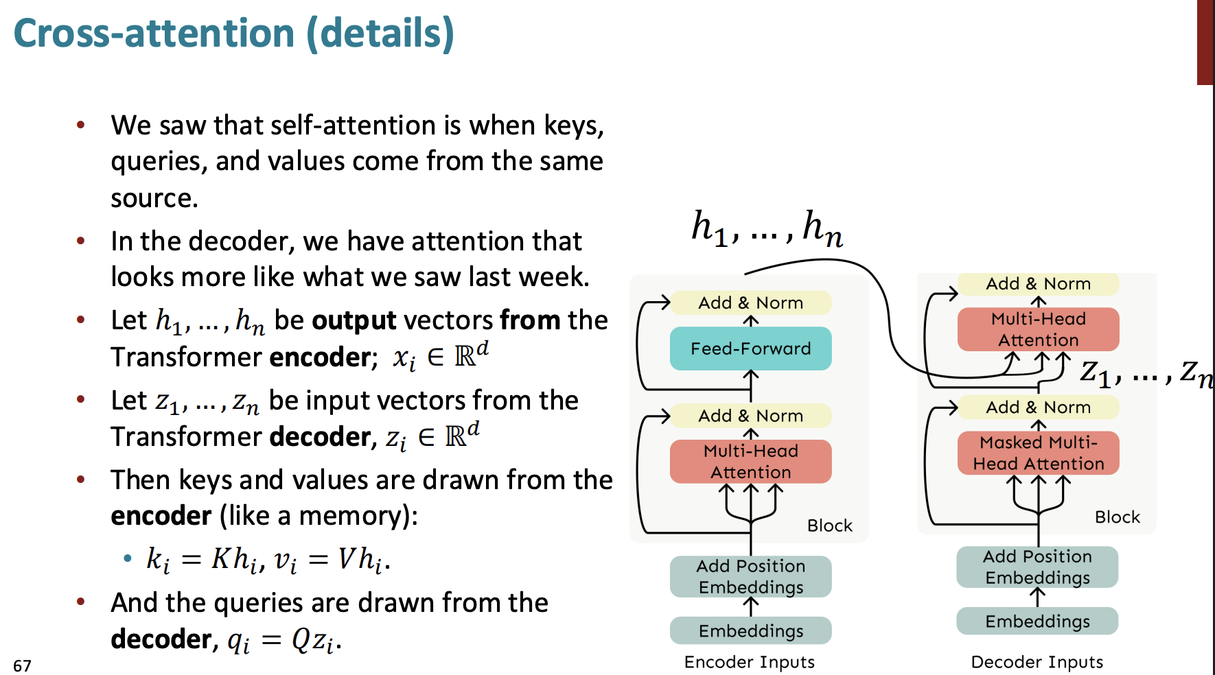
• Also called the seq2seq Transformer
• The Original Transformer, used for machine translation, looks like this

1. source input goes into the encoder
2. target prefix goes into the decoder
3. decoder cross-attends to encoder outputs
4. outputs target token logits
5. computes the cross-entropy loss
6. one backprop pass simultaneously updates the encoder + decoder + embeddings + projection

ViT

ViT = cut the image into patches, treat each patch as a token, and then feed it into the Transformer. Encoder-Only.

• 2d positional encoding
• No masking is used
• For a classification task, one image needs to be represented by a D-dim vector: mean pooling is applied to the output [N, D] matrix, and then a linear layer follows, turning it into a C-dim vector, followed by softmax. (C represents the number of classes)

RL

Markov Decision Process

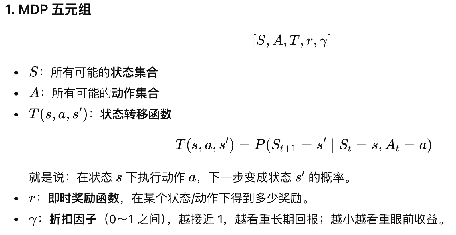
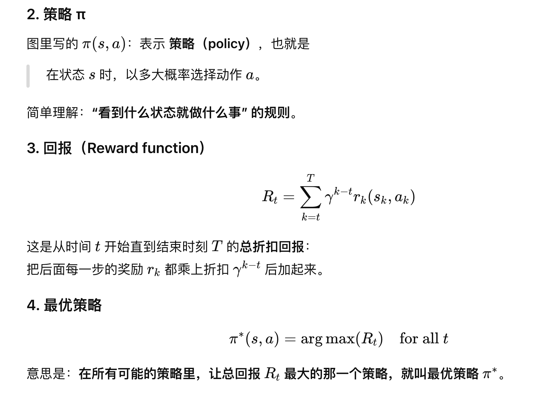A policy needs to be learned

Q-Learning

The meaning of the Q value is: in state s, if we choose action a and then follow policy pi for every subsequent action, this is the expected value of the reward eventually obtained

The initial Q(s,a) is given arbitrarily. For a given state s1, suppose we now know Q(s1,a1),Q(s1,a2),Q(s1,a3),…; we pick the largest Q among them and take the corresponding action, say a3

We hand s1 and a3 to the environment; the environment samples according to the state transition function and returns a new state s’ and an immediate reward r

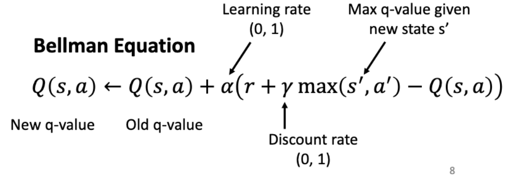
Now that we have the new s’, we can obtain the Q value of the next state and use it to update the current Q(s,a)

Learning rate: how much the new experience will influence or update our current estimate.

Discount rate: if it’s close to 0, we care more about immediate rewards; if it’s close to 1, we also place significant value on future rewards.

DQN

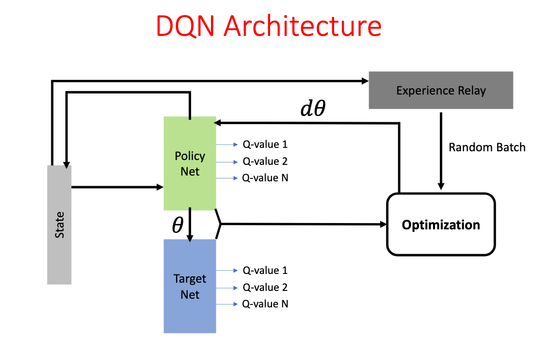
• policy net: takes the current state as input, and outputs the Q-value for each action. Its parameters are updated via back prop
• target net: takes the next state as input, and outputs the Q-value for each action. Its parameters are copied over from the policy net, and are only copied once in a long while
• experience replay: stores a large number of (s, a, r, s’) samples; each training step randomly draws a batch from it
• optimization: randomly draw a batch, compute the loss, and update the policy net’s parameters