ViT

Funnel ViT

paper

Object Detection

slides

Single Object

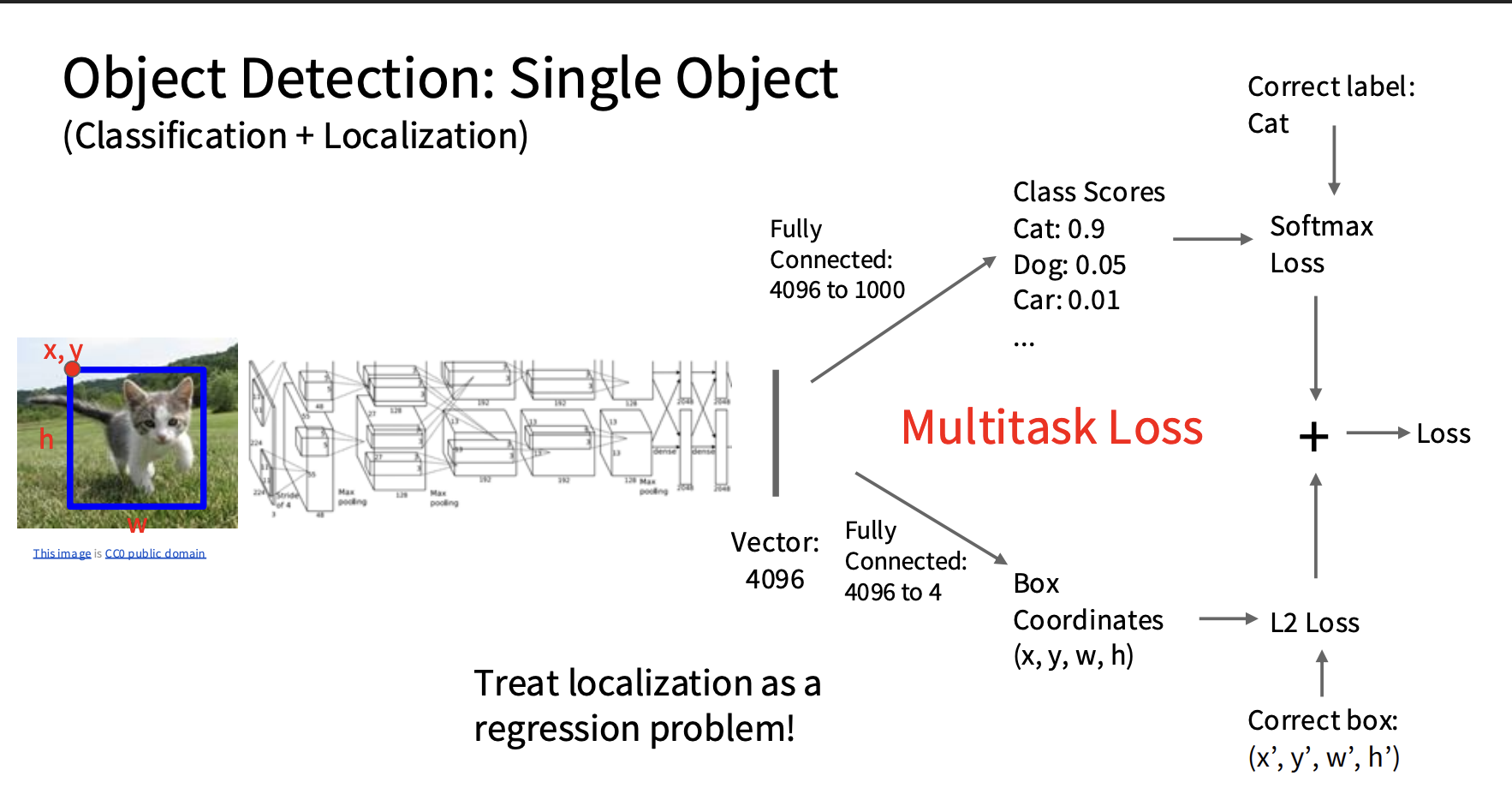
• The label is: Cat + (x’, y’, w’, h')
• x, y = the position of the box’s top-left corner, w = box width, h = box height; these are manually annotated
• The CNN turns the image into a 4096-dim vector
  • classification head: Fully connected, 4096 -> 1000, outputs scores for 1000 classes, then softmax
  • localization head: Fully connected: 4096 -> 4, outputs predicted box = (x, y, w, h); these are continuous values, using L2 loss
  • Total Loss = Softmax Loss + L2 Loss

R-CNN

R-CNN uses Selective Search to generate around 2000 region proposals, warps each proposal to a fixed 224×224 image, then runs a CNN on each region to classify it and later refine the box.

• Selective Search: a traditional CV method
• RoI: candidate region of interest

1. Generate many RoIs
2. Each RoI in the image is cropped out, then resized to 224 x 224, and fed separately into a ConvNet to get many feature vectors
3. For each feature vector:
   • SVMs: determine which class this RoI belongs to (each class outputs one logit)
   • bbox reg: refine this RoI’s box, predicting (dx, dy, dw, dh), i.e., a correction to the previous box

Fast R-CNN

1. First run a CNN backbone on the whole image to get a spatial feature map.

   • The feature map still retains rough positional information; it is not a single vector.

2. Use an external proposal method to get RoIs.

   • In the original Fast R-CNN, RoIs typically come from Selective Search.
   • Note: RPN is an improvement introduced by Faster R-CNN, and is not part of the original Fast R-CNN.

3. Map each RoI onto the feature map, then use RoI Pooling to crop + resize.

   • Different RoIs have different sizes on the feature map.
   • RoI Pooling turns each variable-size RoI feature into a fixed size, e.g., 7×7.
   • This way, the subsequent per-region head can process all RoIs.

4. Make two predictions for each RoI feature:

   • classification: softmax classification, determining object category / background
   • bbox regression: predict box offsets to refine the proposal box

5. Fast R-CNN’s core speedup:

   • R-CNN runs the CNN separately for each RoI.
   • Fast R-CNN runs the CNN only once on the whole image, and all RoIs share the same feature map.

Faster R-CNN

• Faster R-CNN = Fast R-CNN + RPN
• It replaces Selective Search with RPN, making proposal generation learnable as well.

Region Proposal Network

• RPN slides over the backbone feature map.

• At each feature map location, it places multiple anchor boxes.

  • anchor box = a predefined default box
  • Each location can have anchors of multiple scales / aspect ratios

• For each anchor, RPN predicts:

  • objectness: has object / no object
  • box offset: how the anchor should move and scale to get closer to the GT box

• RPN only generates proposals; it is not responsible for the final category classification.

  • It only distinguishes object vs background.
  • The actual category classification is done by the subsequent Fast R-CNN head.

mask R-CNN

Mask R-CNN builds on Faster R-CNN by adding a mask head, responsible for outputting, within this RoI, which pixels belong to the object and which pixels are background

1. A CNN extracts the feature map of the whole image,
2. RPN generates candidate boxes / RoIs on the feature map
3. RoIAlign: crops each RoI out of the feature map and turns it into a fixed size [14,14]; this is the spatial feature map for this RoI
4. For each RoI,

   • the model predicts:

     • C class scores
     • 4 * C sets of box refinements. There are C classes, and each class predicts (dx, dy, dw, dh)

   • RoIAlign outputs a fixed-size RoI feature, e.g. 256 × 14 × 14.

   • The mask head first uses several conv layers to process this RoI feature while keeping the spatial size 14×14.

   • Then a transposed convolution / learnable upsampling layer with stride 2 doubles the spatial resolution:

     • 256 × 14 × 14 -> 256 × 28 × 28

   • Finally, a 1×1 conv maps channels from 256 to C:

     • 256 × 28 × 28 -> C × 28 × 28

   • The output is one 28×28 binary mask per class.

single-stage detector

1. The image is divided into S × S grid cells
2. Each grid cell has three base boxes, B=3, which are anchor boxes of different widths and heights
3. Within each grid cell: Regress from each of the B base boxes to a final box with 5 numbers: (dx, dy, dh, dw, confidence). Predict scores for each of C classes

YOLO

For each box output:

• P(object): probability that the box contains an object
• B bounding boxes (x, y, h, w)
• P(class): probability of belonging to a class

NMS: Non-Maximum Suppression

For a given object, there may be many boxes predicting it. We need to remove the duplicate boxes.

1. Sort all predicted boxes by confidence / class score from high to low.
2. Keep the box with the highest score first. Compute its IoU with the other boxes.
3. If another box’s IoU with it is too high, e.g., IoU > 0.5, that means they are likely detecting the same object, so the lower-scoring box is removed.
4. Repeat this process until all boxes have been processed.

Object Detection with Transformers: DETR

• DETR = Detection Transformer, which models object detection as set prediction.

• Pipeline:

  • image -> CNN backbone -> feature map
  • flatten feature map into image tokens
  • add positional encoding
  • The Transformer encoder processes the image tokens, letting each position see the global context
  • The Transformer decoder receives a set of learned object queries
  • Each object query cross-attends to the encoder output image features inside the Transformer decoder, and finally the decoder outputs a query representation. This representation is then fed into a class head and a box head, producing one object prediction.

• Object queries:

  • Can be understood as a fixed number of object slots, e.g., 100 slots
  • Each query ultimately outputs:
    • class logits: bird / dog / car / … / no-object
    • box coordinates: (cx, cy, w, h)
  • If the image only has 2 objects, then only 2 queries should predict real objects, while the other queries should predict no-object

• Bipartite matching loss:

  • DETR outputs many predicted boxes, but the GT boxes have no order, so predictions and GT need to be matched one-to-one.
  • A matching cost is computed between every predicted box and every GT box.
  • matching cost = classification cost + box L1 cost + GIoU cost
    • IoU measures overlap between predicted and ground-truth boxes.
    • GIoU doesn’t just look at overlap; it also considers how far apart the two boxes are.
  • Hungarian algorithm:
    • Instead of greedily finding the nearest prediction for each GT,
    • it finds a globally minimum-cost one-to-one assignment

• Training after matching:

  • matched predictions:
    • class loss
    • box L1 loss
    • GIoU loss
  • unmatched predictions:
    • no-object classification loss
    • No box loss is computed, since they have no corresponding GT box

Self-supervised learning

231n lecture 12

Pretext tasks from image transformations

Pretext task: not the final task, but a proxy task designed to train the encoder

• rotation: have the model learn to judge how many degrees the image has been rotated. A 4-way classification task.
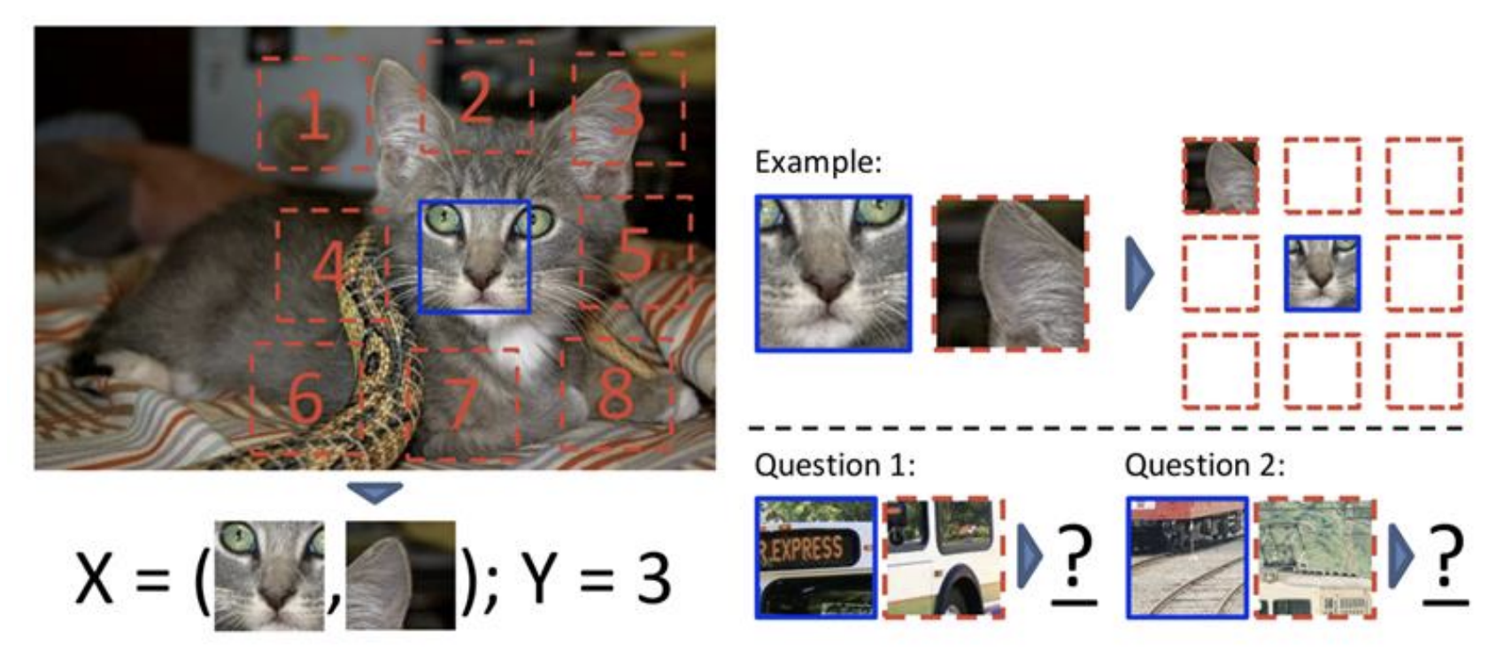
• predict relative patch locations: an 8-class classification task
• Inpainting:

  • Take a complete image x, artificially mask out a region, obtaining a corrupted image.

  • Feed in the corrupted image, and have the model predict the pixels in the masked region.

  • The masked-out region in the original image is the target, so no manual labeling is needed.

  • There are two models:

    • F: the inpainting model / generator, used to fill in the missing region.
    • D: the discriminator, which outputs the probability that “this image is real.”

  • Training is done by alternating:

    1. First use F to generate the completed fake image.
    2. Train D: Use BCE loss to distinguish real images from fake images. real image label = 1 fake image label = 0
    3. Then train F: loss = reconstruction loss + adversarial loss. The reconstruction loss makes the filled-in pixels close to the real pixels. The adversarial loss makes the filled-in image fool D, pushing D(fake) close to 1.

  • Reconstruction loss: Computed only over the masked region, as the gap between predicted pixels and real pixels. The goal is for the content to be correct.

  • Adversarial loss: Essentially a BCE / GAN loss. For D: learn to distinguish real/fake. For F: learn to generate a fake image that fools D into believing it’s real. The goal is to be visually more realistic and less blurry.

Contrastive representation learning

loss: infoNCE

SimCLR

1. For the same image, randomly apply two different augmentations to get x̃_i and x̃_j. During training, pull their embeddings close together.
2. Use the same encoder f to extract features, getting h_i and h_j
3. Use the projection head g to get z_i and z_j
4. Apply the infoNCE loss on z
5. After training, use h as the representation

• h can retain color and texture detail. z mainly retains semantic information, and is used for training

1. Each batch has N images; augmentation produces 2N images
2. For each image, there is 1 positive and (2N-1) negatives
3. When computing the loss, both directions are computed: L = 1/(2N) Σ_{k=1}^N [ l(2k-1, 2k) + l(2k, 2k-1) ]

Gen

Definition

Discriminative Model

Given an input x, which label y does it belong to? Mathematically, this means learning: p(y | x). For example, given a cat image, output the cat/dog label No way to handle unreasonable inputs

Generative Model

Learn: how much does this image itself resemble images that would actually appear in the real world? That is, p(x) = how plausible this image is. Model can “reject” unreasonable inputs by giving them small probability mass.

Conditional Generative Model

Learn p(x | y), e.g., p(image | “cat”), i.e., given the condition is cat, which images look like a cat?

Gen Models

Explicit Density

The model explicitly models p(x), so it can compute the probability/likelihood of an input x.

Autoregressive models

• Can genuinely compute the probability, not just estimate it
• Split x into a sequence, then at each step predict the next element based on the preceding content. Hence it can use the chain rule to explicitly compute p(x).
• LLMs are autoregressive models
• Can also be used to generate images.
  • pixel cnn: given the preceding pixels, what should the value of the current pixel be? Since each pixel has 3 channels with values 0-255, the CNN produces a 256-dim softmax representing the probability distribution over the next pixel’s value
  • p(x) = p(x1) * p(x2 | x1) * p(x3 | x1, x2) * …, which lets it learn the probability of the whole image

Approximate density

Want to model p(x), but can only compute it approximately. Use a hidden space z to represent the underlying factors behind the data, then generate x from z

(Non-Variational) Autoencoders

• An autoencoder is a reconstruction problem.
• Input image x goes through the Encoder to get a latent representation z, then goes through the Decoder to reconstruct x_hat.
• x -> Encoder -> z -> Decoder -> x_hat
• loss = ||x_hat - x||^2, i.e., making the reconstructed image as close to the original as possible.
• Backprop updates the parameters of both the Encoder and the Decoder at the same time; the Encoder can be thought of as the first half of the model, and the Decoder as the second half.
• The z in the middle is the learned representation / compressed feature.
• If z has a bottleneck, e.g., a smaller dimensionality, the model is forced to retain only the information most useful for reconstruction, so z may learn factors such as object identity, appearance, and scene layout.

Problem: The logic of a plain autoencoder is that if we can generate a z, then the decoder can generate an image from it. But the key issue is that it’s hard to learn to generate a meaningful z

VAE

Variational Autoencoders (VAE) define an intractable density that we cannot explicitly compute or optimize

But we will be able to directly optimize a lower bound on the density

• training data: x
• intuition: maximize pθ(x), i.e., the probability / density that these training images would be generated under the current model pθ

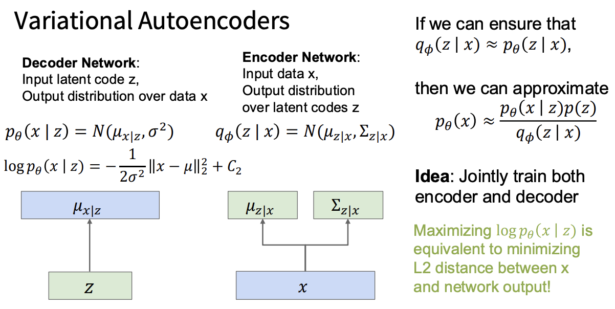
• decoder:

  • input z, output μ_{x|z}
  • learn pθ(x | z) = N(μ_{x|z}, σ²)
  • if image: 28*28 pixels, then output 784 means; when generating an image, the means are usually used directly
  • Assume all pixels share the same fixed variance σ²

• encoder:

  • learn qφ(z | x) = N(μ_{z|x}, Σ_{z|x}), which approximates p(z|x)
  • input x, output μ_{z|x}, Σ_{z|x}
  • Σ = diagonal vector; this only accounts for each pixel having its own variance, without modeling the correlation between different pixels.

• use bayes to calculate p(x)=p(x|z)*p(z)/p(z|x)

• want to maximize p(x) <=> loss function=-log(p(x))

• training

  • The first two terms are called the ELBO, and the third term is called the gap. Since KL>=0, the ELBO is a lower bound on the loss. During training, only the first two terms are optimized.
  • First term: the reconstruction term. Given an x, sample many z’s from the distribution learned by the encoder, and for each z compute log(p(x|z)), i.e., feed z to the decoder and see how likely the decoder is to reconstruct the original x, then average these results. The purpose of this term is to train the model’s reconstruction ability, making the encoder and decoder better.
  • Second term: - D_KL(qφ(z|x) || p(z)). At generation time, z is sampled directly from a predefined z distribution, usually N(0, I). Here p(z) is the prior distribution; during training, p(z) is assumed to follow a standard Gaussian. The purpose of this term is that each sample’s qφ(z|x) is regularized to not stray too far from p(z). This way, once trained, we can sample z directly from p(z) and use the decoder to generate new images. KL represents how dissimilar two distributions are
  • Third term: + D_KL(qφ(z|x) || pθ(z|x)). Note that pθ(z|x) is the true posterior. It represents: if we have already seen image x, then under the current decoder, which z’s are most likely to have generated this x? We use the encoder qφ(z|x) to approximate the true posterior. Since pθ(z|x) cannot be computed, this third term cannot be computed either

• summary: Jointly train encoder q and decoder p to maximize the variational lower bound on the data likelihood

Implicit Density

Does not explicitly compute p(x)

Generative Adversarial Network (GAN)

slides

give up on modeling p(x), but allow us to draw samples from p(x)

1. Sample z from p(z), usually z ~ N(0, I)

2. Generate fake images: fake = G(z)

3. Sample real images x from the training dataset: x ~ p_data

4. Send both real images x and fake images G(z) to the discriminator: D(x) = probability real image is real D(G(z)) = probability fake image is real

5. Freeze Generator, update Discriminator: maximize: E_{xp_data}[log D(x)] + E_{zp(z)}[log(1 - D(G(z)))]

   In words: D should output 1 for real images, and 0 for fake images.

6. Freeze Discriminator, update Generator: sample new z ~ p(z), fake = G(z), send fake to D

   Generator wants: D(G(z)) -> 1

   In words: G wants to fool D into thinking fake images are real.

Ideally, D(x) ≈ 0.5, meaning D cannot tell whether the images generated by the Generator are real or fake

VQGAN

VQGAN = VQ-VAE + GAN loss; it trains four models: Encoder + Codebook + Decoder + Discriminator

• VQ: Vector Quantization, meaning the latent is discrete, e.g., z=[14, 302, 81, 7, 999, …]
• codebook=[e1, e2, e3], each vector is a high-dimensional continuous vector representing one kind of feature. Learnable parameters

1. Image x goes through the encoder to get a spatial latent grid z_e, e.g., [2,2,3], 4 locations in total, each location being a 3-dim vector

2. For each 3-dim vector, find the nearest vector in the codebook, then assign this vector a token id. Finally, this image’s feature is flattened into z_tokens = [0, 1, 0, 2]

3. Look up the codebook to get z_q (a continuous vector), then feed it to the decoder to get the reconstructed image, x_hat

4. Let the discriminator distinguish real / reconstructed

Why does VQGAN add a GAN loss?

If only a reconstruction loss is used, e.g., L2 / MSE, the reconstructed image tends to be blurry, because MSE encourages the model to output an “average answer.” The role of the GAN loss is to make the reconstructed image visually resemble a real photo, with sharp texture

How is it trained

A. Update Encoder + Codebook + Decoder B. Update Discriminator

Diffusion

noise -> denoise -> denoise -> … -> image

Diffusion

cs 231n lecture 14

training

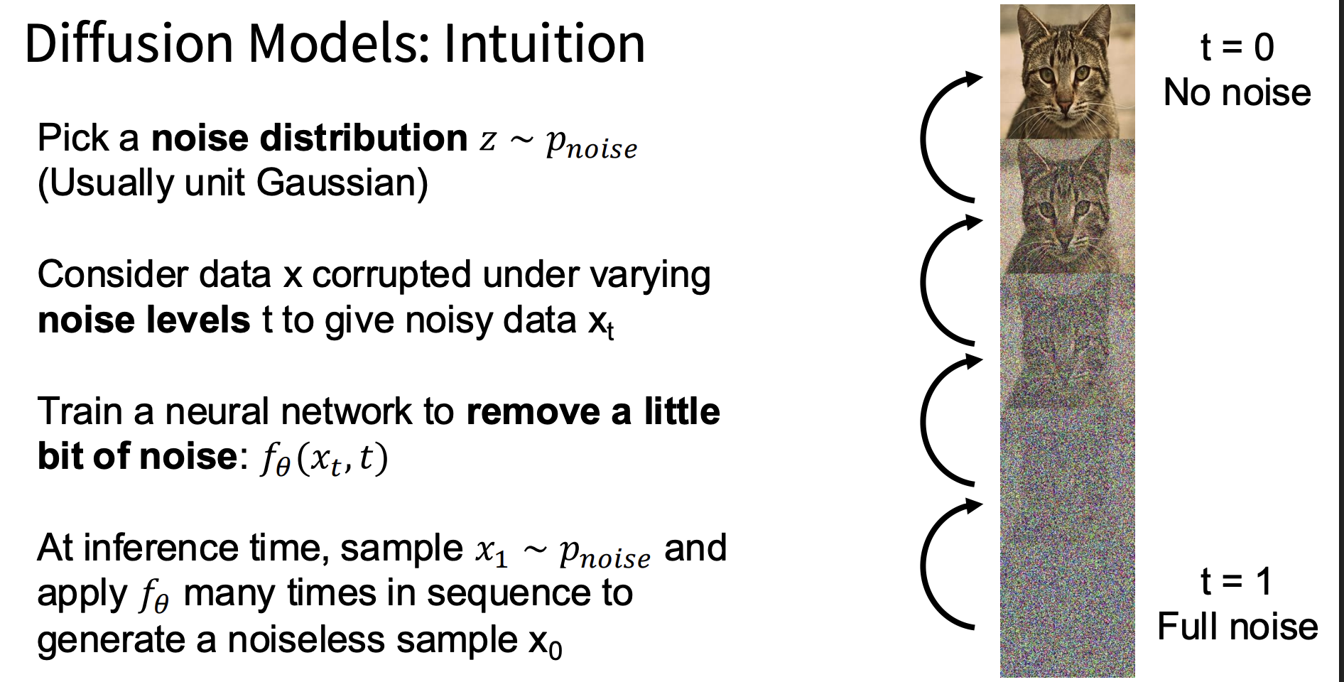
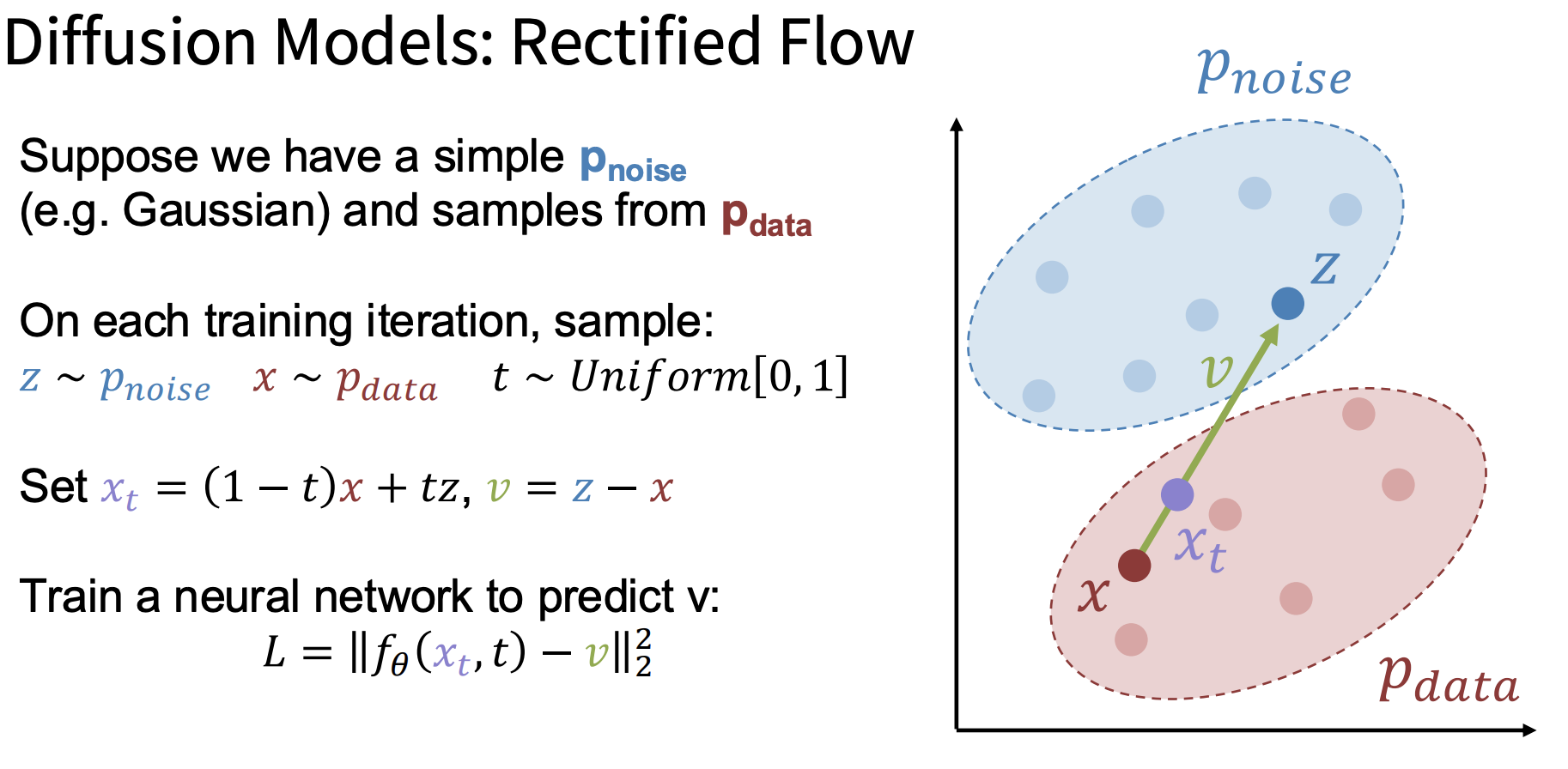
1. Sample a z from a unit Gaussian, representing noise
2. Sample a real image x and a time t, and generate an image x_t that is t steps along the path from noise to the real image
3. Train an NN so it learns to predict v = z - x, i.e., learn the direction from the real image to noise

inference

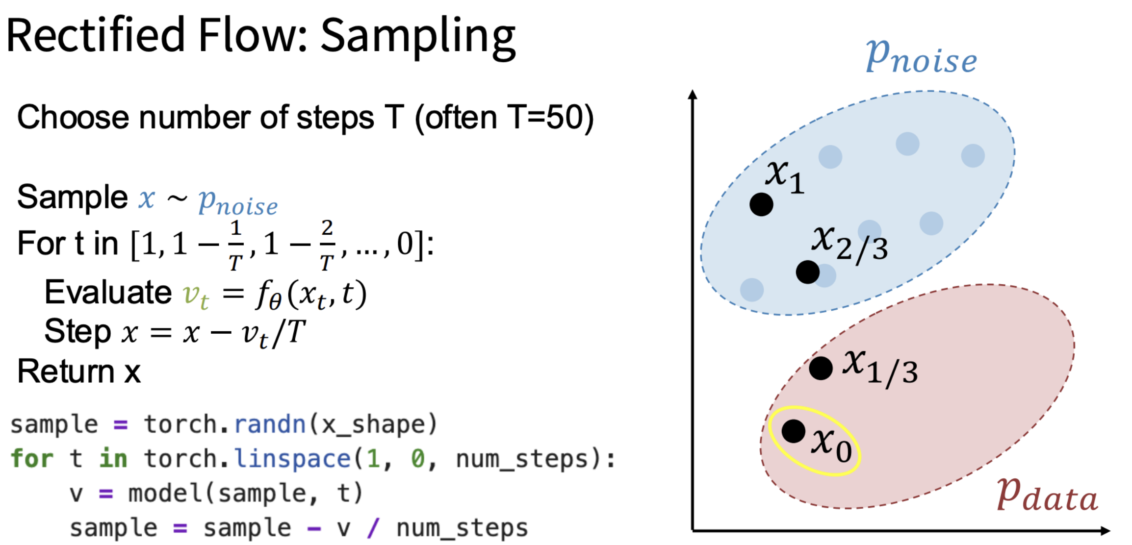
1. Sample a noise
2. Starting from t=1, use the model to predict v at this step (input the current image and t)
3. Move in the direction opposite to v, updating the image. This is the denoising process.

Conditional

Generate a data sample matching condition y, starting from pure noise

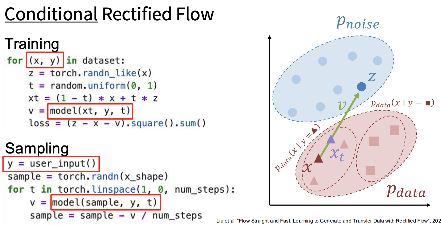
• During training, samples look like (x, y)
  • x: an image of a cat
  • y: “cat”
• The large red region is all real data: Pdata
• But within it, it can be divided into many smaller regions: Pdata(x∣y)
• Let the model learn to move to the correct region

cfg

Strengthening the prompt’s constraint

• During training, randomly set the condition y=null; this gives the model both the ability to follow the prompt and the general ability to generate realistic images
• At inference time, for a given intermediate image, two v’s are predicted separately: one without a specified prompt, and one with a specified prompt
• Compute v_cfg = v_y + w*(v_y - v_null); this diff represents the direction contributed by the condition. So this is done to amplify that direction to make the generation follow the prompt more strongly

Latent Diffusion Model

Instead of doing diffusion directly on the raw image pixels, first compress the image into a latent, do diffusion on the latent, and finally decode it back into an image.

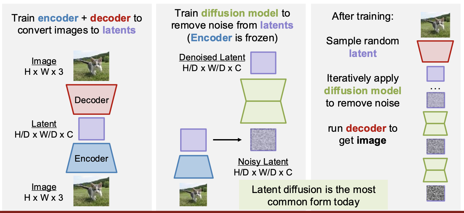
Training

• Train an encoder-decoder with a VAE to learn the latent
• Train diffusion on the latent

Inference

• Sample a random latent noise
• Use diffusion to remove noise from the latent
• Use the decoder to generate an image from the latent

Diffusion Transformer (DiT)

DiT replaces the network responsible for denoising inside the diffusion model, swapping U-Net for a Transformer

timestamp condition

• The timestamp enters a condition MLP; the scale / shift it outputs there dynamically replace the fixed, learned γ / β in an ordinary LayerNorm.
• α1, α2: control the residual

  1 2 3

  h = AdaLN(x) attn_out = SelfAttention(h) x = x + α1 * attn_out

token condition(cross attention)

• Q: noisy image latent tokens
• K/V: text tokens

token condition(joint attention)

• Concatenate the condition tokens and the input tokens together, and feed them into the Transformer

MMDiT

• image tokens and text tokens each have their own modality-specific Q/K/V projections.

• image tokens -> Q_img, K_img, V_img

• text tokens -> Q_txt, K_txt, V_txt

• Then concatenate Q/K/V along the sequence dimension: Q = [Q_img; Q_txt] K = [K_img; K_txt] V = [V_img; V_txt]

• Perform one joint attention using the concatenated Q/K/V.

• The attention output is then split back into the image stream and the text stream.

• In the end, only the output corresponding to the target image tokens goes through the output head, and is mapped to the denoising direction v.

• text tokens / reference image tokens are the condition context, they participate in attention, but are not decoded into the final image by the VAE decoder.

text-to-image

1. The text prompt is first turned into text embeddings
2. Generate a noisy latent
3. DiT takes the text embeddings and noisy latent as input, and outputs a clean latent
4. The decoder restores the latent into the output image