0%

https://medium.com/pinterest-engineering/building-pinterest-canvas-a-text-to-image-foundation-model-aa34965e84d9

https://arxiv.org/abs/2603.06453?utm_source=chatgpt.com

https://github.com/junfanz1/Awesome-AI-Review/blob/main/System%20Design/GenAI%20System%20Design.md#5-text-to-image

Pinterest Canvas

Text-To-Image

Generate images conditioned on both text prompts and reference images.

1. text-to-image

  • Inference
    1. Embed the text prompt to obtain the text embedding
    2. Feed the noisy target latent and the text embedding into the DiT together to obtain the clean target latent
    3. The clean target latent passes through the VAE decoder to produce the image
  • Training
    • Training data: (text prompt, real image)
    • Only the DiT is trained. Both the text encoder and the VAE use pretrained weights, and are then frozen
    • The real image passes through the VAE encoder to obtain the real latent. During training, x_t is generated from the real latent

2. multimodal image editing tasks

Stage 2 starts from the trained Stage 1 text-to-image model.

bytebytego tutorial

dataset

  • A query image
  • (n-1) negative images
  • A positive image, i.e., the image most similar to the query image.
  • The index label of the positive image among all the images.

build dataset

  • human judgement: humans annotate the most similar image
  • user interaction
    • noisy
    • sparse: may not have click data available for lots of the images
  • generate similar images

Offline metrics

Mean reciprocal rank (MRR)

MRR=1/m * sum(1/rank_i)

Neural Network

terminology

For example, suppose there are 10,000 samples with a batch size of 100:

  • epoch: all 10,000 samples go through forward + back prop once. After every epoch, the data should be shuffled to make sure each batch is made up of a different combination of samples each time.

  • iteration: one iteration means 100 samples go through one forward pass (computing the loss) + backpropagation (computing the gradients), and then optimizer.step() updates the weights.

CLIP

paper

 1
 2
 3
 4
 5
 6
 7
 8
 9
10
11
12
13
14
15
16
17
18
19
20
# image_encoder - ResNet or Vision Transformer
# text_encoder - CBOW or Text Transformer
# I[n, h, w, c] - minibatch of aligned images
# T[n, l] - minibatch of aligned texts
# W_i[d_i, d_e] - learned proj of image to embed
# W_t[d_t, d_e] - learned proj of text to embed
# t - learned temperature parameter
# extract feature representations of each modality
I_f = image_encoder(I) #[n, d_i]
T_f = text_encoder(T) #[n, d_t]
# joint multimodal embedding [n, d_e]
I_e = l2_normalize(np.dot(I_f, W_i), axis=1) #[n, d_e]
T_e = l2_normalize(np.dot(T_f, W_t), axis=1) #[n, n]
# scaled pairwise cosine similarities [n, n]
logits = np.dot(I_e, T_e.T) * np.exp(t)
# symmetric loss function
labels = np.arange(n)
loss_i = cross_entropy_loss(logits, labels, axis=1) # image-to-text loss
loss_t = cross_entropy_loss(logits, labels, axis=0)
loss = (loss_i + loss_t)/2

architecture

image encoder

VisionTransformer
  • Input: [B,3,H,W]
  • Output: [B,output_dim]
 1
 2
 3
 4
 5
 6
 7
 8
 9
10
11
12
13
14
15
16
17
18
19
20
21
22
23
24
25
26
27
28
29
30
31
32
33
34
35
36
class VisionTransformer(nn.Module):
    def __init__(self, input_resolution: int, patch_size: int, width: int, layers: int, heads: int, output_dim: int):
        super().__init__()
        self.input_resolution = input_resolution
        self.output_dim = output_dim
        self.conv1 = nn.Conv2d(in_channels=3, out_channels=width, kernel_size=patch_size, stride=patch_size, bias=False) #width is the hidden dimension of each token in the Transformer.
        # grid=input_resolution/patch_size
        # after conv1, becomes [B, width, grid, grid]
        scale = width ** -0.5
        self.class_embedding = nn.Parameter(scale * torch.randn(width)) #class token, a special token dedicated to "collecting information from the whole image"
        self.positional_embedding = nn.Parameter(scale * torch.randn((input_resolution // patch_size) ** 2 + 1, width)) # [(input_resolution // patch_size) ** 2 + 1, width]
        self.ln_pre = LayerNorm(width)

        self.transformer = Transformer(width, layers, heads)

        self.ln_post = LayerNorm(width)
        self.proj = nn.Parameter(scale * torch.randn(width, output_dim))

    def forward(self, x: torch.Tensor):
        x = self.conv1(x)  # shape = [*, width, grid, grid]
        x = x.reshape(x.shape[0], x.shape[1], -1)  # shape = [*, width, grid ** 2]
        x = x.permute(0, 2, 1)  # shape = [*, grid ** 2, width]
        x = torch.cat([self.class_embedding.to(x.dtype) + torch.zeros(x.shape[0], 1, x.shape[-1], dtype=x.dtype, device=x.device), x], dim=1)  # shape = [*, grid ** 2 + 1, width]
        x = x + self.positional_embedding.to(x.dtype)
        x = self.ln_pre(x)

        x = x.permute(1, 0, 2)  # NLD -> LND
        x = self.transformer(x)
        x = x.permute(1, 0, 2)  # LND -> NLD

        x = self.ln_post(x[:, 0, :])

        if self.proj is not None:
            x = x @ self.proj

        return x

text encoder

embedding space

ViT

Funnel ViT

paper

Object Detection

slides

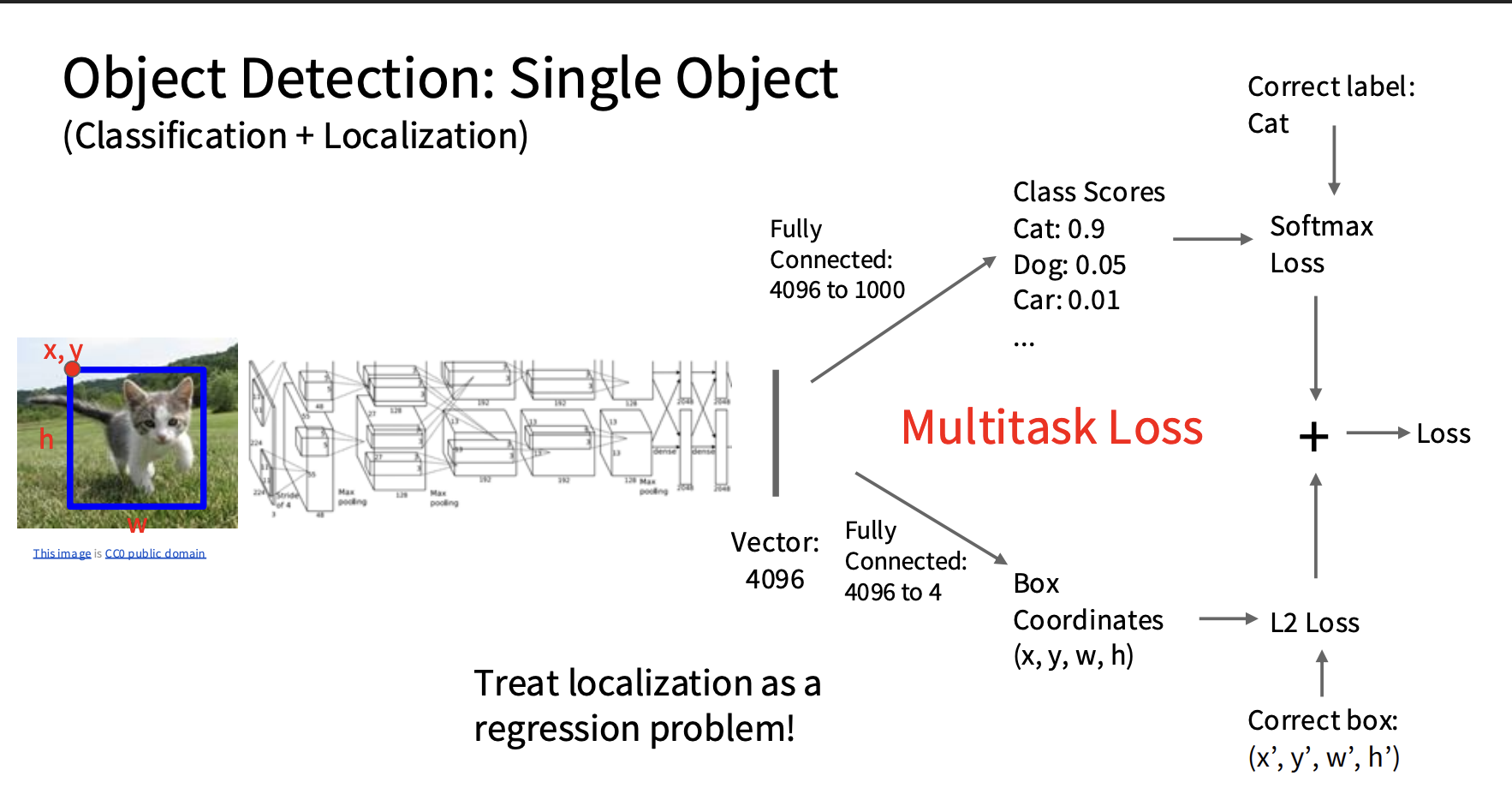
Single Object

alt text

  • The label is: Cat + (x’, y’, w’, h')
  • x, y = the position of the box’s top-left corner, w = box width, h = box height; these are manually annotated
  • The CNN turns the image into a 4096-dim vector
    • classification head: Fully connected, 4096 -> 1000, outputs scores for 1000 classes, then softmax
    • localization head: Fully connected: 4096 -> 4, outputs predicted box = (x, y, w, h); these are continuous values, using L2 loss
    • Total Loss = Softmax Loss + L2 Loss

R-CNN

R-CNN uses Selective Search to generate around 2000 region proposals, warps each proposal to a fixed 224×224 image, then runs a CNN on each region to classify it and later refine the box.

https://github.com/andrewekhalel/MLQuestions https://www.1point3acres.com/bbs/forum.php?mod=viewthread&tid=998257&page=1&extra= https://longxingtan.gitbook.io/mle-interview/02_ml

supervised learning

training data includes both the input features and corresponding target labels

classification

Logistic Regression

linear classification, binary classification loss function: Binary Cross-Entropy Loss

alt text alt text

Does logistic regression have a closed-form solution?

No, there is no closed-form solution. Although the loss function is convex, taking its derivative yields a nonlinear equation containing an exponential term, so we cannot set the derivative to 0 and solve for closed-form expressions of w and b; we can only use gradient descent.

Module

The parent class of all models; every network inherits from it

  • init(self)
  • forward(self, x)

conv

Bilibili

1
output=F.conv2d(input, kernel, stride=1) # performs the convolution computation, producing the feature matrix

Conv2d

 1
 2
 3
 4
 5
 6
 7
 8
 9
10
11
12
13
14
15
16
17
18
19
20
21
22
23
24
25
26
27
28
import torch
import torch.nn as nn

class CNN(nn.Module):
    def __init__(self):
        super().__init__()

        self.conv1 = nn.Conv2d(
            in_channels=3,
            out_channels=6,
            kernel_size=3,
            stride=1,
            padding=0
        )

        self.maxpool1 = nn.MaxPool2d(
            kernel_size=3,  # Pooling window size: 3×3
            ceil_mode=True  # Ceiling mode, keeps incomplete edge windows
            # stride defaults to kernel_size=3; you can also explicitly write stride=3, with exactly the same effect
        )

    def forward(self, x):
        # Forward pass: **first convolve to extract features, then pool to downsample** (standard CNN order)
        # x: [b, 3, h, w]
        x = self.conv1(x)       # Step 1: pass through the conv layer, producing a 6-channel feature map, [b, 6, h', w']
        # h'=(h+2*p-k)/s+1
        x = self.maxpool1(x)    # Step 2: pass through the pooling layer, downsampling the feature map
        return x

Linear

1
2
3
4
5
self.linear = nn.Linear(
    in_features=1024,
    out_features=512,
    bias=True        # Default True; whether to add the bias b
)

weight = (512, 1024) bias = (512) y = x @ W.T + b

RPC Basics

protobuf IDL

  1. Define the .proto file: define Request/Response formats and function signatures.
  2. Protobuf generates CalculatorStub automatically.
    1
    2
    3
    4
    5
    6
    7
    8
    
    channel = grpc.insecure_channel("server-ip:port")
    
    # Client stub (a local proxy for server-side methods)
    stub = CalculatorStub(channel)
    
    # Call Stub.Add as if it were a local function
    request = AddRequest(num1=2, num2=3)
    response = stub.Add(request)
  3. Implement the actual logic for add on the server side.

Semantics

At most once

Common Operations

x.bit_count(): Returns the number of 1s in the binary representation of x. Can also be interpreted as the minimum number of powers of 2 needed to represent x.

Brain Teasers

2749. Minimum Operations to Make the Integer Zero

Let x = num1 - k * num2, then the problem transforms to: Can x be represented using k powers of 2 (duplicates allowed)?

Find the upper and lower bounds of x and enumerate. Plot x = num1 - k * num2 with k as x-axis and x as y-axis. The answer lies in some points on this line in the first quadrant. Analyze the equation x=2^(i1)+…2^(ik) to find possible x values.

Prime Numbers

Sieve of Eratosthenes

1
2
3
4
5
6
7
8
9
# Time complexity O(MX * log log MX)
MX = 1_000_001
is_prime = [False] * 2 + [True] * (MX - 2)  # 0 and 1 are not prime
primes = []
for i in range(2, MX):
    if is_prime[i]:
        primes.append(i)
        for j in range(i * i, MX, i):
            is_prime[j] = False  # j is a multiple of prime i

204. Count Primes

p[i] represents the number of primes less than or equal to i. Starting from i=2, p[i]==0 <=> i is prime. Then, starting from ii, mark multiples of i as composite (by setting p[ik]=-1). And, p[i] is assigned p[i-1]+1.